Tutorial: Building the IWFM Sample Model from Scratch#
This tutorial demonstrates how to build the official IWFM sample model programmatically with pyiwfm and then run it. The sample model is a uniform grid with homogeneous aquifer properties, streams, a lake, root zone land use, and a 10-year daily simulation.
Learning Objectives#
By the end of this tutorial, you will be able to:
Create mesh nodes and elements programmatically
Define stratigraphy layers
Configure groundwater, stream, lake, and root zone components
Assemble an
IWFMModeland write all input filesRun the IWFM preprocessor and simulation
Visualize simulation results
Overview#
The IWFM sample model we are building has these properties:
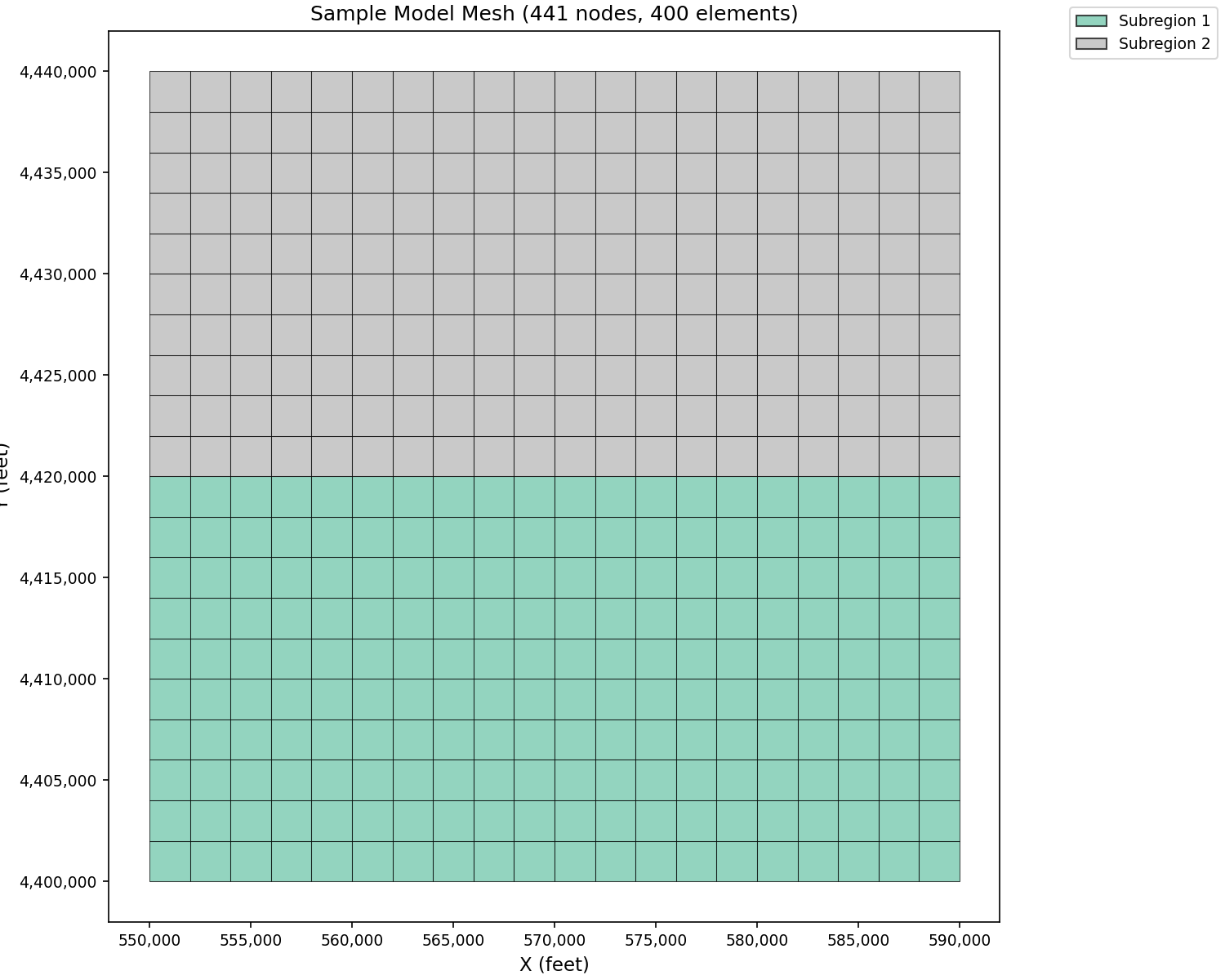
Mesh: 21 x 21 rectangular grid (441 nodes, 400 quad elements)
Subregions: 2 (south half and north half)
Stratigraphy: 2 aquifer layers
Streams: 3 reaches with 23 stream nodes
Lakes: 1 lake
Root Zone: 2 nonponded crops + 5 ponded crops (7 crop types)
Simulation period: 10/01/1990 – 09/30/2000 (daily timestep)
Section 1: Create the Mesh#
Build the 21 x 21 node grid (441 nodes) and 400 quadrilateral elements:
import numpy as np
from pyiwfm.core.mesh import AppGrid, Node, Element, Subregion

# Grid dimensions
nx, ny = 21, 21
x0, y0 = 550_000.0, 4_400_000.0   # Lower-left corner
dx, dy = 2_000.0, 2_000.0          # Node spacing (square elements)

# Create nodes
nodes = {}
node_id = 1
for j in range(ny):
    for i in range(nx):
        is_boundary = (i == 0 or i == nx - 1 or j == 0 or j == ny - 1)
        nodes[node_id] = Node(
            id=node_id,
            x=x0 + i * dx,
            y=y0 + j * dy,
            is_boundary=is_boundary,
        )
        node_id += 1

print(f"Created {len(nodes)} nodes")

# Create elements (20 x 20 = 400 quads)
elements = {}
elem_id = 1
for j in range(ny - 1):
    for i in range(nx - 1):
        n1 = j * nx + i + 1
        n2 = n1 + 1
        n3 = n2 + nx
        n4 = n1 + nx
        # South half = subregion 1, north half = subregion 2
        subregion = 1 if j < 10 else 2
        elements[elem_id] = Element(
            id=elem_id,
            vertices=(n1, n2, n3, n4),
            subregion=subregion,
        )
        elem_id += 1

print(f"Created {len(elements)} elements")

# Subregion definitions
subregions = {
    1: Subregion(id=1, name="Region1"),
    2: Subregion(id=2, name="Region2"),
}

# Assemble the grid
grid = AppGrid(nodes=nodes, elements=elements, subregions=subregions)
grid.compute_connectivity()

print(f"Grid: {grid.n_nodes} nodes, {grid.n_elements} elements")
print(f"Subregions: {sorted(grid.subregions)}")
Here is what the mesh looks like with subregions colored:
import matplotlib.pyplot as plt
from pyiwfm.sample_models import build_tutorial_model
from pyiwfm.visualization.plotting import plot_elements

m = build_tutorial_model()
fig, ax = plot_elements(m.grid, color_by='subregion', cmap='Set2')

ax.set_title(f'Sample Model Mesh ({m.grid.n_nodes} nodes, {m.grid.n_elements} elements)')
ax.set_xlabel('X (feet)')
ax.set_ylabel('Y (feet)')
plt.show()
Section 2: Define Stratigraphy#
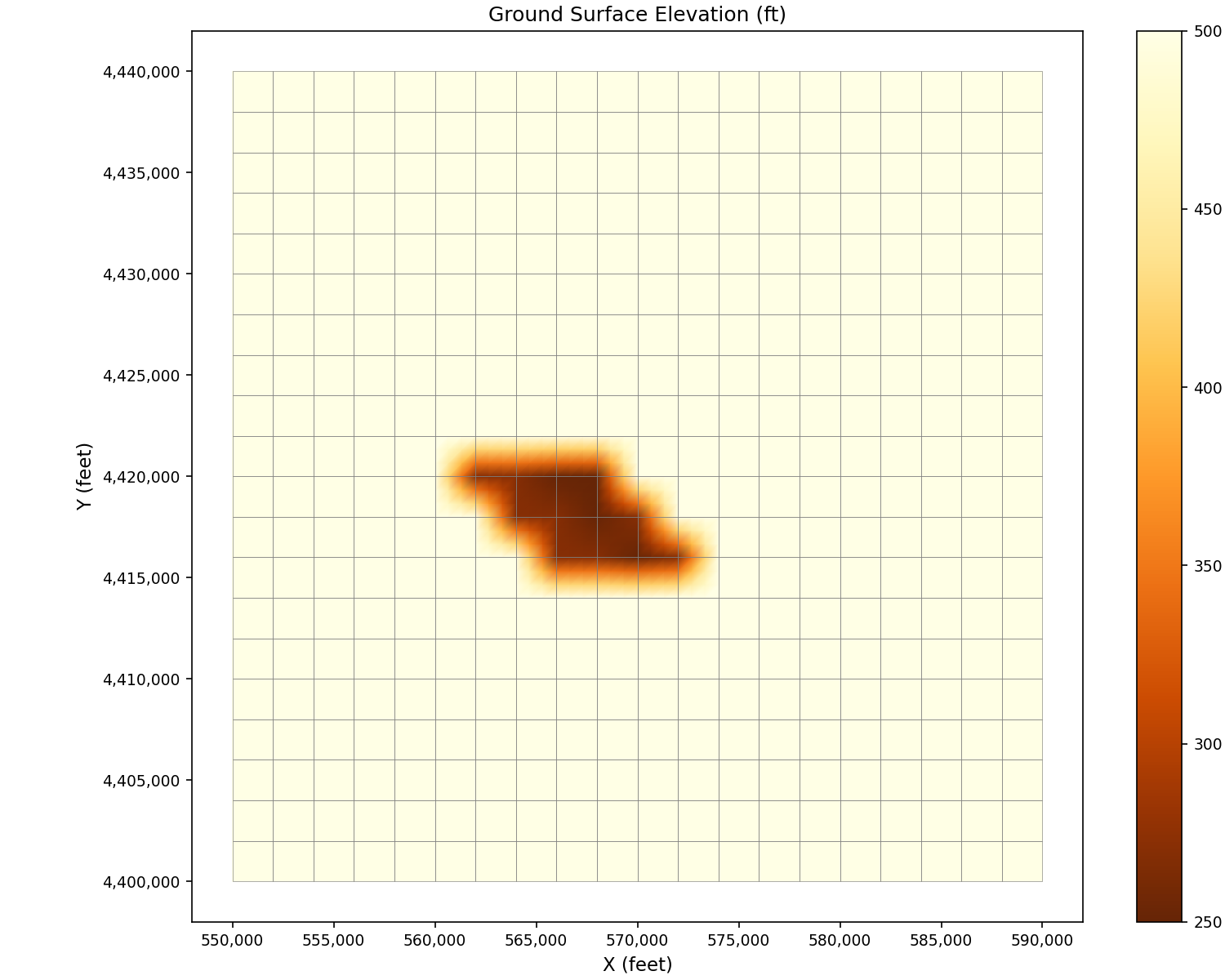
Create a 2-layer stratigraphy. The ground surface is mostly flat at 500 ft, with a depression where the lake bed sits:
from pyiwfm.core.stratigraphy import Stratigraphy

n_nodes = grid.n_nodes
n_layers = 2

# Ground surface elevation: 500 ft everywhere, with lake-bed depression
gs_elev = np.full(n_nodes, 500.0)

# Lower elevations around the lake area (nodes from the Strata.dat)
for nid in [177, 178, 180, 197, 198, 200, 217, 218]:
    gs_elev[nid - 1] = 270.0
for nid in [179, 199, 219, 220]:
    gs_elev[nid - 1] = 250.0

# Layer 1: aquifer extends from ground surface down to elevation 0
top_elev_l1 = gs_elev.copy()
bottom_elev_l1 = np.zeros(n_nodes)

# Layer 2: 10-ft confining layer for nodes 1-231, then 100-ft aquifer
confining = np.zeros(n_nodes)
confining[:231] = 10.0
top_elev_l2 = bottom_elev_l1 - confining
bottom_elev_l2 = top_elev_l2 - 100.0

top_elev = np.column_stack([top_elev_l1, top_elev_l2])
bottom_elev = np.column_stack([bottom_elev_l1, bottom_elev_l2])
active_node = np.ones((n_nodes, n_layers), dtype=bool)

stratigraphy = Stratigraphy(
    n_layers=n_layers,
    n_nodes=n_nodes,
    gs_elev=gs_elev,
    top_elev=top_elev,
    bottom_elev=bottom_elev,
    active_node=active_node,
)

print(f"Stratigraphy: {stratigraphy.n_layers} layers")
print(f"Ground surface range: {gs_elev.min():.0f} - {gs_elev.max():.0f} ft")
Visualize ground surface elevation:
import matplotlib.pyplot as plt
from pyiwfm.sample_models import build_tutorial_model
from pyiwfm.visualization.plotting import plot_scalar_field

m = build_tutorial_model()
fig, ax = plot_scalar_field(m.grid, m.gs_elev, field_type='node', cmap='YlOrBr_r',
                            show_mesh=True, edge_color='gray')

ax.set_title('Ground Surface Elevation (ft)')
ax.set_xlabel('X (feet)')
ax.set_ylabel('Y (feet)')
plt.show()
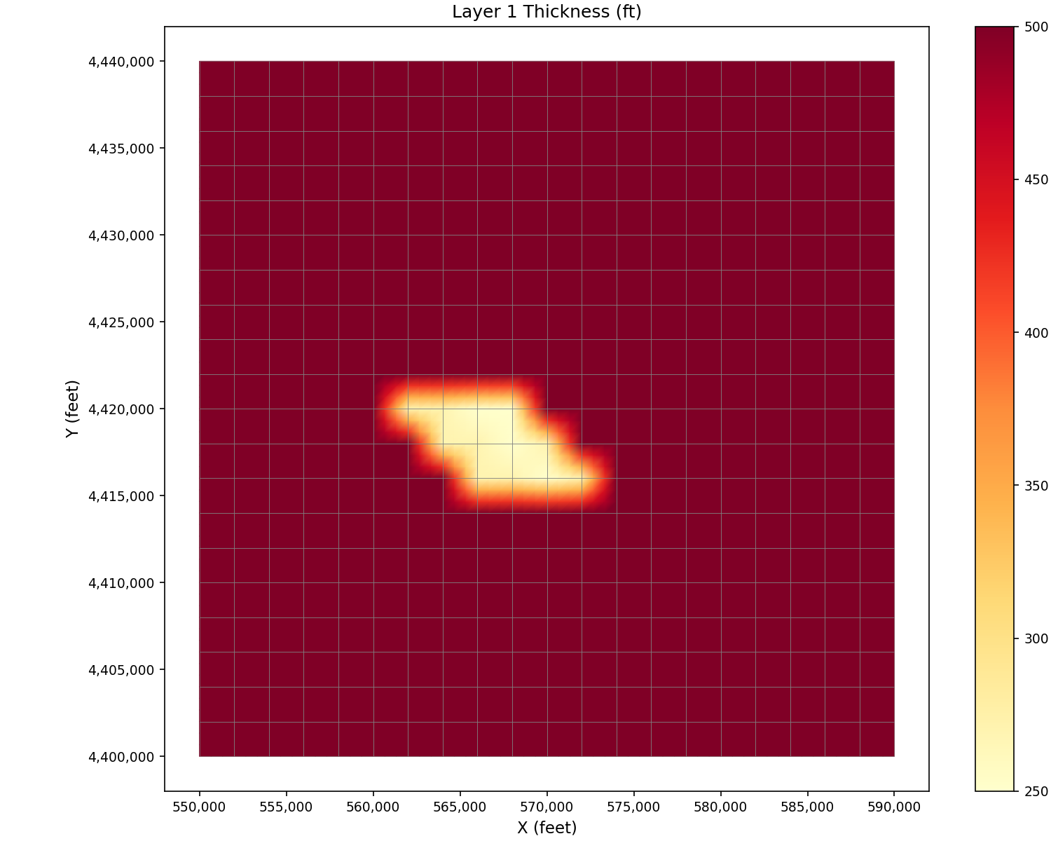
Visualize layer thickness:
import matplotlib.pyplot as plt
from pyiwfm.sample_models import build_tutorial_model
from pyiwfm.visualization.plotting import plot_scalar_field

m = build_tutorial_model()
thickness = m.stratigraphy.top_elev[:, 0] - m.stratigraphy.bottom_elev[:, 0]
fig, ax = plot_scalar_field(m.grid, thickness, field_type='node', cmap='YlOrRd')

ax.set_title('Layer 1 Thickness (ft)')
ax.set_xlabel('X (feet)')
ax.set_ylabel('Y (feet)')
plt.show()
Section 3: Groundwater Component#
Configure the groundwater component with aquifer parameters, initial heads, and boundary conditions:
from pyiwfm.components.groundwater import (
AppGW, AquiferParameters, BoundaryCondition,
ElementPumping, TileDrain, NodeSubsidence, HydrographLocation,
)
n_layers = 2
# Aquifer parameters (uniform across all nodes and layers)
aquifer_params = AquiferParameters(
n_nodes=n_nodes,
n_layers=n_layers,
kh=np.full((n_nodes, n_layers), 50.0), # Horiz. K (ft/day)
kv=np.full((n_nodes, n_layers), 1.0), # Vert. K (ft/day)
specific_storage=np.full((n_nodes, n_layers), 1e-6),
specific_yield=np.full((n_nodes, n_layers), 0.25),
aquitard_kv=np.full((n_nodes, n_layers), 0.2),
)
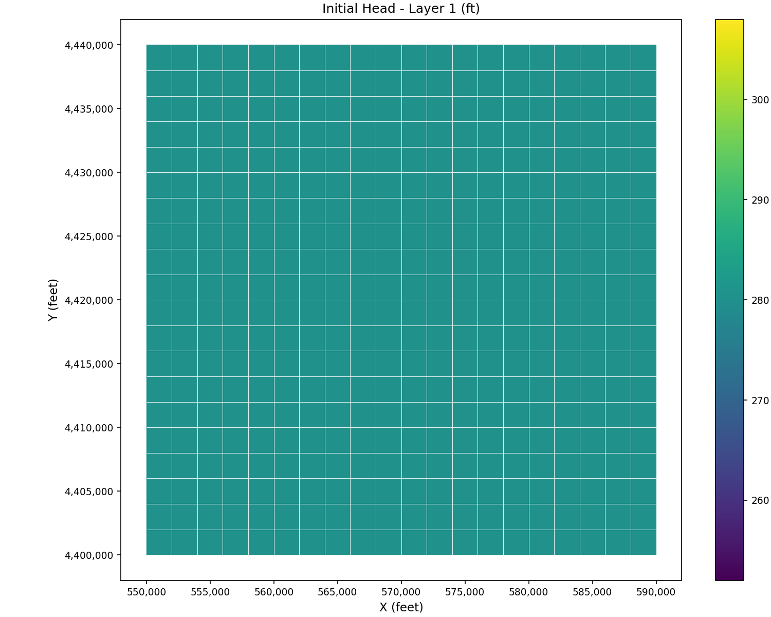
# Initial heads: uniform 280 (layer 1) and 290 (layer 2)
initial_heads = np.column_stack([
np.full(n_nodes, 280.0),
np.full(n_nodes, 290.0),
])
# West boundary: 21 nodes, constant specified head = 290
west_nodes = [j * nx + 1 for j in range(ny)]
bc_west = BoundaryCondition(
id=1, bc_type="specified_head",
nodes=west_nodes, values=[290.0] * len(west_nodes), layer=1,
)
# East boundary: 21 nodes, time-series driven
east_nodes = [j * nx + nx for j in range(ny)]
bc_east = BoundaryCondition(
id=2, bc_type="specified_head",
nodes=east_nodes, values=[290.0] * len(east_nodes), layer=1,
ts_column=1,
)
# Element pumping: 5 wells
element_pumping = [
ElementPumping(element_id=73, layer=1, pump_rate=0.0, pump_column=1),
ElementPumping(element_id=193, layer=1, pump_rate=0.0, pump_column=2),
ElementPumping(element_id=333, layer=1, pump_rate=0.0, pump_column=3),
ElementPumping(element_id=134, layer=2, pump_rate=0.0, pump_column=4),
ElementPumping(element_id=274, layer=2, pump_rate=0.0, pump_column=5),
]
# Tile drains: 21 drains along column 6 (1-based: node 6, 27, 48, ...)
tile_drains = {}
for td_i in range(ny):
td_node = td_i * nx + 6
td_id = td_i + 1
tile_drains[td_id] = TileDrain(
id=td_id, element=td_node, elevation=280.0,
conductance=20_000.0, destination_type="stream", destination_id=20,
)
# Node subsidence: uniform parameters for all nodes
node_subsidence = [
NodeSubsidence(
node_id=nid,
elastic_sc=[5e-6, 5e-6], inelastic_sc=[5e-5, 5e-5],
interbed_thick=[10.0, 10.0], interbed_thick_min=[2.0, 2.0],
)
for nid in range(1, n_nodes + 1)
]
# Hydrograph locations: center column, both layers
center_col = 11 # 1-based column index
hydrograph_locations = []
for j in range(ny):
hyd_nid = j * nx + center_col
for layer in range(1, n_layers + 1):
hydrograph_locations.append(HydrographLocation(
node_id=hyd_nid, layer=layer,
x=nodes[hyd_nid].x, y=nodes[hyd_nid].y,
name=f"Obs_N{hyd_nid}_L{layer}",
))
# Assemble groundwater component
gw = AppGW(
n_nodes=n_nodes, n_layers=n_layers, n_elements=grid.n_elements,
aquifer_params=aquifer_params, heads=initial_heads,
boundary_conditions=[bc_west, bc_east],
element_pumping=element_pumping, tile_drains=tile_drains,
node_subsidence=node_subsidence, hydrograph_locations=hydrograph_locations,
)
print(f"GW: {len(gw.boundary_conditions)} BCs, "
f"{len(gw.element_pumping)} pumps, "
f"{len(gw.tile_drains)} tile drains, "
f"{len(gw.hydrograph_locations)} hydrograph locations")
Visualize initial head distribution:
import matplotlib.pyplot as plt
from pyiwfm.sample_models import build_tutorial_model
from pyiwfm.visualization.plotting import plot_scalar_field

m = build_tutorial_model()
fig, ax = plot_scalar_field(m.grid, m.initial_heads[:, 0], field_type='node',
                            cmap='viridis', show_mesh=True, edge_color='white')

ax.set_title('Initial Head - Layer 1 (ft)')
ax.set_xlabel('X (feet)')
ax.set_ylabel('Y (feet)')
plt.show()
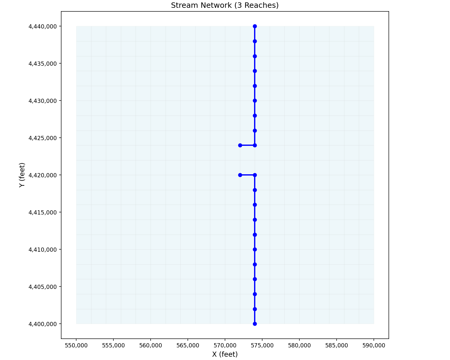
Section 4: Stream Component#
Create the stream network with 3 reaches and 23 stream nodes. The groundwater node mapping follows the official IWFM sample model, with Reach 1 flowing from north to south, then Reaches 2 and 3 branching:
from pyiwfm.components.stream import (
    AppStream, StrmNode, StrmReach, Diversion, Bypass,
)

stream = AppStream()

# GW node mapping for each stream node (from Stream.dat)
reach1_gw = [433, 412, 391, 370, 349, 328, 307, 286, 265, 264]
reach2_gw = [222, 223, 202, 181, 160, 139]
reach3_gw = [139, 118, 97, 76, 55, 34, 13]
all_gw = reach1_gw + reach2_gw + reach3_gw

# Stream bottom elevations decline 2 ft per node
bottom_elevs = [300.0 - 2.0 * i for i in range(23)]

for sid, gw_nid in enumerate(all_gw, start=1):
    stream.add_node(StrmNode(
        id=sid, gw_node=gw_nid,
        x=nodes[gw_nid].x, y=nodes[gw_nid].y,
        bottom_elev=bottom_elevs[sid - 1],
        conductivity=10.0, bed_thickness=1.0, wetted_perimeter=150.0,
    ))

# 3 reaches
stream.add_reach(StrmReach(id=1, upstream_node=1, downstream_node=10,
                            nodes=list(range(1, 11))))
stream.add_reach(StrmReach(id=2, upstream_node=11, downstream_node=16,
                            nodes=list(range(11, 17))))
stream.add_reach(StrmReach(id=3, upstream_node=17, downstream_node=23,
                            nodes=list(range(17, 24))))

# 5 diversions
stream.add_diversion(Diversion(id=1, source_node=3,  destination_type="element",
                                destination_id=152, name="Div1", max_div_column=1))
stream.add_diversion(Diversion(id=2, source_node=5,  destination_type="element",
                                destination_id=128, name="Div2", max_div_column=2))
stream.add_diversion(Diversion(id=3, source_node=8,  destination_type="element",
                                destination_id=65,  name="Div3", max_div_column=3))
stream.add_diversion(Diversion(id=4, source_node=13, destination_type="element",
                                destination_id=181, name="Div4", max_div_column=4))
stream.add_diversion(Diversion(id=5, source_node=20, destination_type="element",
                                destination_id=55,  name="Div5", max_div_column=5))

# 2 bypasses (second has a rating table)
stream.add_bypass(Bypass(id=1, source_node=10, destination_node=11,
                          name="Bypass1", capacity=500.0))
stream.add_bypass(Bypass(id=2, source_node=16, destination_node=17,
                          name="Bypass2", capacity=1000.0,
                          rating_table_flows=[0.0, 500.0, 1000.0, 2000.0],
                          rating_table_spills=[0.0, 100.0, 300.0, 800.0]))

print(f"Streams: {stream.n_nodes} nodes, {stream.n_reaches} reaches, "
      f"{len(stream.diversions)} diversions, {len(stream.bypasses)} bypasses")
Visualize the stream network overlaid on the mesh:
import matplotlib.pyplot as plt
from pyiwfm.sample_models import build_tutorial_model
from pyiwfm.visualization.plotting import plot_mesh, plot_streams

m = build_tutorial_model()
fig, ax = plot_mesh(m.grid, show_edges=True, edge_color='lightgray', alpha=0.2)
plot_streams(m.stream, ax=ax, show_nodes=True, line_width=2)

ax.set_title('Stream Network (3 Reaches)')
ax.set_xlabel('X (feet)')
ax.set_ylabel('Y (feet)')
plt.show()
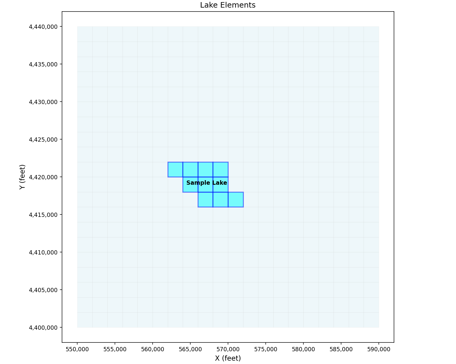
Section 5: Lake Component#
Define a lake occupying 10 elements in the upper-center of the domain (matching the official sample model’s Lake.dat):
from pyiwfm.components.lake import AppLake, Lake, LakeElement, LakeOutflow

lake_component = AppLake()

lake = Lake(
    id=1,
    name="Sample Lake",
    max_elevation=350.0,
    initial_elevation=280.0,
    bed_conductivity=2.0,
    bed_thickness=1.0,
    et_column=7,
    precip_column=2,
    max_elev_column=1,
    outflow=LakeOutflow(
        lake_id=1, destination_type="stream", destination_id=10,
    ),
)
lake_component.add_lake(lake)

# 10 lake elements (from Lake.dat)
lake_elem_ids = [169, 170, 171, 188, 189, 190, 207, 208, 209, 210]
for eid in lake_elem_ids:
    lake_component.add_lake_element(LakeElement(lake_id=1, element_id=eid))

print(f"Lakes: {len(lake_component.lakes)} lake(s), "
      f"{len(lake_component.lake_elements)} elements")
Visualize lake elements highlighted on the mesh:
import matplotlib.pyplot as plt
from pyiwfm.sample_models import build_tutorial_model
from pyiwfm.visualization.plotting import plot_mesh, plot_lakes

m = build_tutorial_model()
fig, ax = plot_mesh(m.grid, show_edges=True, edge_color='lightgray', alpha=0.2)
plot_lakes(m.lakes, m.grid, ax=ax)

ax.set_title('Lake Elements')
ax.set_xlabel('X (feet)')
ax.set_ylabel('Y (feet)')
plt.show()
Section 6: Root Zone Component#
Configure root zone with non-ponded crops (tomato, alfalfa) and ponded crops (rice varieties, refuge):
from pyiwfm.components.rootzone import RootZone, CropType, SoilParameters

rz = RootZone(n_elements=grid.n_elements, n_layers=n_layers)

# Define crop types with root depths (ft)
# 2 nonponded + 5 ponded = 7 crop types (matching IWFM sample model)
crops = [
    CropType(id=1, name="TO",         root_depth=5.0),  # Tomato (nonponded)
    CropType(id=2, name="AL",         root_depth=6.0),  # Alfalfa (nonponded)
    CropType(id=3, name="RICE_FL",    root_depth=3.0),  # Rice - fully irrigated
    CropType(id=4, name="RICE_NFL",   root_depth=3.0),  # Rice - not fully irrigated
    CropType(id=5, name="RICE_NDC",   root_depth=3.0),  # Rice - no decomposition
    CropType(id=6, name="REFUGE_SL",  root_depth=3.0),  # Refuge - seasonal
    CropType(id=7, name="REFUGE_PR",  root_depth=3.0),  # Refuge - permanent
]
for crop in crops:
    rz.add_crop_type(crop)

# Sandy soils: elements 1-200 (south half, subregion 1)
for eid in range(1, 201):
    rz.set_soil_parameters(eid, SoilParameters(
        porosity=0.45, field_capacity=0.20, wilting_point=0.0,
        saturated_kv=2.60, lambda_param=0.62,
    ))

# Clay soils: elements 201-400 (north half, subregion 2)
for eid in range(201, 401):
    rz.set_soil_parameters(eid, SoilParameters(
        porosity=0.50, field_capacity=0.33, wilting_point=0.0,
        saturated_kv=0.68, lambda_param=0.36,
    ))

print(f"Root Zone: {len(rz.crop_types)} crop types, "
      f"{len(rz.soil_params)} element soil params")
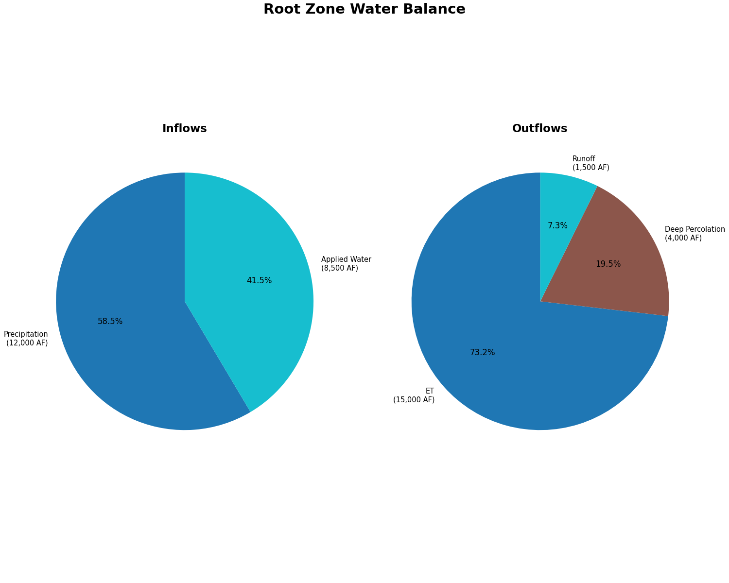
Visualize the root zone water balance as a pie chart:
import matplotlib.pyplot as plt
from pyiwfm.sample_models import build_tutorial_model
from pyiwfm.visualization.plotting import plot_budget_pie

m = build_tutorial_model()
fig, ax = plot_budget_pie(m.rz_budget, title='Root Zone Water Balance',
                           budget_type='both')
plt.show()
Section 7: Assemble and Write the Model#
Combine all components into an IWFMModel and write to disk:
from pathlib import Path
from pyiwfm.core.model import IWFMModel
from pyiwfm.io import save_complete_model

# Assemble the model
model = IWFMModel(
    name="IWFM Sample Model",
    mesh=grid,
    stratigraphy=stratigraphy,
    groundwater=gw,
    streams=stream,
    lakes=lake_component,
    rootzone=rz,
    metadata={
        "start_date": "10/01/1990",
        "end_date": "09/30/2000",
        "timestep": "1DAY",
    },
)

print(model.summary())

# Write all input files
output_dir = Path("sample_model_output")
output_dir.mkdir(exist_ok=True)

files_written = save_complete_model(model, output_dir)

print(f"\nFiles written ({len(files_written)}):")
for name, path in sorted(files_written.items()):
    print(f"  {name}: {path}")
Section 8: Run the Preprocessor#
Use IWFMRunner to execute the IWFM preprocessor:
from pyiwfm.runner.runner import IWFMRunner
from pyiwfm.runner.executables import find_iwfm_executables

# Find IWFM executables on the system
executables = find_iwfm_executables()
print(f"Preprocessor: {executables.preprocessor}")
print(f"Simulation:   {executables.simulation}")

# Run preprocessor
runner = IWFMRunner(executables=executables, working_dir=output_dir)
pp_result = runner.run_preprocessor("Preprocessor.in")

print(f"Preprocessor success: {pp_result.success}")
if not pp_result.success:
    print(f"Error: {pp_result.stderr}")
else:
    print("Preprocessor completed successfully")
Section 9: Run the Simulation#
Execute the IWFM simulation:
sim_result = runner.run_simulation("Simulation.in", timeout=600)

print(f"Simulation success: {sim_result.success}")
if sim_result.success:
    print(f"Runtime: {sim_result.runtime:.1f} seconds")
    print("Output files generated")
else:
    print(f"Error: {sim_result.stderr}")
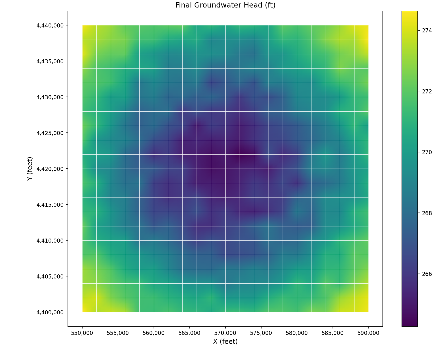
Section 10: Visualize Results#
Load and visualize the simulation results. The examples below use sample data to demonstrate what each plot looks like:
Groundwater heads at final timestep:
import matplotlib.pyplot as plt
from pyiwfm.sample_models import build_tutorial_model
from pyiwfm.visualization.plotting import plot_scalar_field

m = build_tutorial_model()
fig, ax = plot_scalar_field(m.grid, m.final_heads, field_type='node',
                            cmap='viridis', show_mesh=True, edge_color='white')

ax.set_title('Final Groundwater Head (ft)')
ax.set_xlabel('X (feet)')
ax.set_ylabel('Y (feet)')
plt.show()
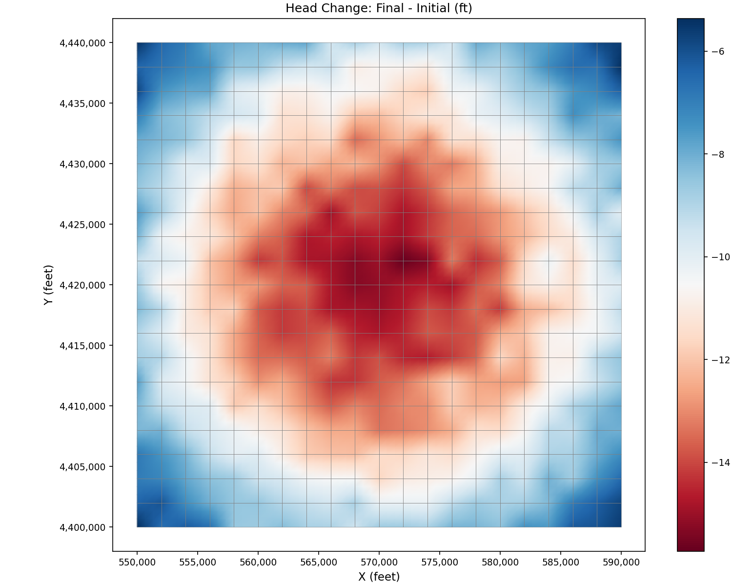
Head change (final minus initial):
import matplotlib.pyplot as plt
from pyiwfm.sample_models import build_tutorial_model
from pyiwfm.visualization.plotting import plot_scalar_field

m = build_tutorial_model()
head_change = m.final_heads - m.initial_heads[:, 0]
fig, ax = plot_scalar_field(m.grid, head_change, field_type='node', cmap='RdBu')

ax.set_title('Head Change: Final - Initial (ft)')
ax.set_xlabel('X (feet)')
ax.set_ylabel('Y (feet)')
plt.show()
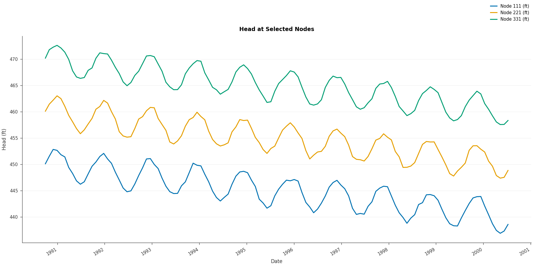
Head time series at selected nodes:
import matplotlib.pyplot as plt
from pyiwfm.sample_models import build_tutorial_model
from pyiwfm.visualization.plotting import plot_timeseries

m = build_tutorial_model()
fig, ax = plot_timeseries(m.head_timeseries, title='Head at Selected Nodes',
                           ylabel='Head (ft)')
plt.show()
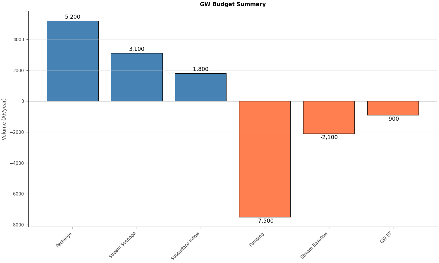
Groundwater budget summary:
import matplotlib.pyplot as plt
from pyiwfm.sample_models import build_tutorial_model
from pyiwfm.visualization.plotting import plot_budget_bar

m = build_tutorial_model()
fig, ax = plot_budget_bar(m.gw_budget, title='GW Budget Summary',
                           units='AF/year')
plt.show()
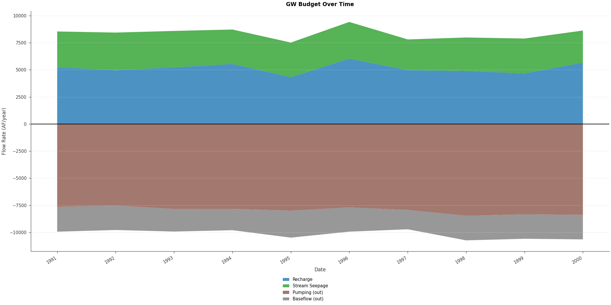
Budget over time:
import matplotlib.pyplot as plt
from pyiwfm.sample_models import build_tutorial_model
from pyiwfm.visualization.plotting import plot_budget_stacked

m = build_tutorial_model()
budget_times, budget_components = m.gw_budget_timeseries
fig, ax = plot_budget_stacked(budget_times, budget_components,
                               title='GW Budget Over Time', units='AF/year')
plt.show()
Root zone water balance:
import matplotlib.pyplot as plt
from pyiwfm.sample_models import build_tutorial_model
from pyiwfm.visualization.plotting import plot_budget_pie

m = build_tutorial_model()
fig, ax = plot_budget_pie(m.rz_budget, title='Root Zone Water Balance',
                           budget_type='both')
plt.show()

Interactive Viewing#
For interactive 3D visualization and map exploration, launch the web viewer:
pyiwfm viewer --model-dir sample_model_output/
This opens a browser with 4 tabs: Overview, 3D Mesh, Results Map, and Budgets.
Complete Script#
Here is the complete script combining all steps:
"""Build the IWFM sample model from scratch and visualize results."""

import numpy as np
from pathlib import Path
from pyiwfm.core.mesh import AppGrid, Node, Element, Subregion
from pyiwfm.core.stratigraphy import Stratigraphy
from pyiwfm.core.model import IWFMModel
from pyiwfm.components.groundwater import (
    AppGW, AquiferParameters, BoundaryCondition,
    ElementPumping, TileDrain, NodeSubsidence, HydrographLocation,
)
from pyiwfm.components.stream import (
    AppStream, StrmNode, StrmReach, Diversion, Bypass,
)
from pyiwfm.components.lake import AppLake, Lake, LakeElement, LakeOutflow
from pyiwfm.components.rootzone import RootZone, CropType, SoilParameters
from pyiwfm.io import save_complete_model
from pyiwfm.visualization.plotting import (
    plot_mesh, plot_elements, plot_scalar_field, plot_streams, plot_lakes,
    plot_timeseries, plot_budget_bar,
)

# ---- 1. Mesh ----
nx, ny = 21, 21
x0, y0 = 550_000.0, 4_400_000.0
dx, dy = 2_000.0, 2_000.0

nodes = {}
nid = 1
for j in range(ny):
    for i in range(nx):
        is_boundary = (i == 0 or i == nx - 1 or j == 0 or j == ny - 1)
        nodes[nid] = Node(id=nid, x=x0 + i * dx, y=y0 + j * dy,
                          is_boundary=is_boundary)
        nid += 1

elements = {}
eid = 1
for j in range(ny - 1):
    for i in range(nx - 1):
        n1 = j * nx + i + 1
        elements[eid] = Element(
            id=eid,
            vertices=(n1, n1 + 1, n1 + 1 + nx, n1 + nx),
            subregion=1 if j < 10 else 2,
        )
        eid += 1

subregions = {1: Subregion(id=1, name="Region1"),
              2: Subregion(id=2, name="Region2")}
grid = AppGrid(nodes=nodes, elements=elements, subregions=subregions)
grid.compute_connectivity()

# ---- 2. Stratigraphy ----
n_nodes = grid.n_nodes
n_layers = 2
gs_elev = np.full(n_nodes, 500.0)
for nid in [177, 178, 180, 197, 198, 200, 217, 218]:
    gs_elev[nid - 1] = 270.0
for nid in [179, 199, 219, 220]:
    gs_elev[nid - 1] = 250.0

top_elev_l1 = gs_elev.copy()
bottom_elev_l1 = np.zeros(n_nodes)
confining = np.zeros(n_nodes)
confining[:231] = 10.0
top_elev_l2 = bottom_elev_l1 - confining
bottom_elev_l2 = top_elev_l2 - 100.0

stratigraphy = Stratigraphy(
    n_layers=2, n_nodes=n_nodes, gs_elev=gs_elev,
    top_elev=np.column_stack([top_elev_l1, top_elev_l2]),
    bottom_elev=np.column_stack([bottom_elev_l1, bottom_elev_l2]),
    active_node=np.ones((n_nodes, 2), dtype=bool),
)

# ---- 3. Groundwater ----
initial_heads = np.column_stack([
    np.full(n_nodes, 280.0), np.full(n_nodes, 290.0),
])
aquifer_params = AquiferParameters(
    n_nodes=n_nodes, n_layers=n_layers,
    kh=np.full((n_nodes, n_layers), 50.0),
    kv=np.full((n_nodes, n_layers), 1.0),
    specific_storage=np.full((n_nodes, n_layers), 1e-6),
    specific_yield=np.full((n_nodes, n_layers), 0.25),
    aquitard_kv=np.full((n_nodes, n_layers), 0.2),
)
west_nodes = [j * nx + 1 for j in range(ny)]
east_nodes = [j * nx + nx for j in range(ny)]
gw = AppGW(
    n_nodes=n_nodes, n_layers=n_layers, n_elements=grid.n_elements,
    aquifer_params=aquifer_params, heads=initial_heads,
    boundary_conditions=[
        BoundaryCondition(id=1, bc_type="specified_head",
                          nodes=west_nodes, values=[290.0]*len(west_nodes), layer=1),
        BoundaryCondition(id=2, bc_type="specified_head",
                          nodes=east_nodes, values=[290.0]*len(east_nodes),
                          layer=1, ts_column=1),
    ],
    element_pumping=[
        ElementPumping(element_id=e, layer=l, pump_rate=0.0, pump_column=c)
        for e, l, c in [(73,1,1),(193,1,2),(333,1,3),(134,2,4),(274,2,5)]
    ],
    tile_drains={
        i+1: TileDrain(id=i+1, element=i*nx+6, elevation=280.0,
                        conductance=20_000.0, destination_type="stream",
                        destination_id=20)
        for i in range(ny)
    },
    node_subsidence=[
        NodeSubsidence(node_id=n, elastic_sc=[5e-6,5e-6],
                       inelastic_sc=[5e-5,5e-5],
                       interbed_thick=[10.0,10.0],
                       interbed_thick_min=[2.0,2.0])
        for n in range(1, n_nodes+1)
    ],
    hydrograph_locations=[
        HydrographLocation(node_id=j*nx+11, layer=lay,
                            x=nodes[j*nx+11].x, y=nodes[j*nx+11].y,
                            name=f"Obs_N{j*nx+11}_L{lay}")
        for j in range(ny) for lay in range(1, n_layers+1)
    ],
)

# ---- 4. Streams ----
stream = AppStream()
reach1_gw = [433, 412, 391, 370, 349, 328, 307, 286, 265, 264]
reach2_gw = [222, 223, 202, 181, 160, 139]
reach3_gw = [139, 118, 97, 76, 55, 34, 13]
all_gw = reach1_gw + reach2_gw + reach3_gw
bottom_elevs = [300.0 - 2.0 * i for i in range(23)]
for sid, gw_nid in enumerate(all_gw, start=1):
    stream.add_node(StrmNode(id=sid, gw_node=gw_nid,
                             x=nodes[gw_nid].x, y=nodes[gw_nid].y,
                             bottom_elev=bottom_elevs[sid - 1],
                             conductivity=10.0, bed_thickness=1.0,
                             wetted_perimeter=150.0))
stream.add_reach(StrmReach(id=1, upstream_node=1, downstream_node=10,
                            nodes=list(range(1, 11))))
stream.add_reach(StrmReach(id=2, upstream_node=11, downstream_node=16,
                            nodes=list(range(11, 17))))
stream.add_reach(StrmReach(id=3, upstream_node=17, downstream_node=23,
                            nodes=list(range(17, 24))))
for did, sn, de in [(1,3,152),(2,5,128),(3,8,65),(4,13,181),(5,20,55)]:
    stream.add_diversion(Diversion(id=did, source_node=sn,
                                    destination_type="element",
                                    destination_id=de,
                                    name=f"Div{did}", max_div_column=did))
stream.add_bypass(Bypass(id=1, source_node=10, destination_node=11,
                          name="Bypass1", capacity=500.0))
stream.add_bypass(Bypass(id=2, source_node=16, destination_node=17,
                          name="Bypass2", capacity=1000.0,
                          rating_table_flows=[0.0, 500.0, 1000.0, 2000.0],
                          rating_table_spills=[0.0, 100.0, 300.0, 800.0]))

# ---- 5. Lake ----
lake_comp = AppLake()
lake_comp.add_lake(Lake(id=1, name="Sample Lake", max_elevation=350.0,
                         initial_elevation=280.0, bed_conductivity=2.0,
                         bed_thickness=1.0, et_column=7, precip_column=2,
                         max_elev_column=1,
                         outflow=LakeOutflow(lake_id=1,
                                              destination_type="stream",
                                              destination_id=10)))
for lake_eid in [169, 170, 171, 188, 189, 190, 207, 208, 209, 210]:
    lake_comp.add_lake_element(LakeElement(lake_id=1, element_id=lake_eid))

# ---- 6. Root Zone ----
rz = RootZone(n_elements=grid.n_elements, n_layers=n_layers)
for crop in [CropType(id=1, name="TO", root_depth=5.0),
             CropType(id=2, name="AL", root_depth=6.0),
             CropType(id=3, name="RICE_FL", root_depth=3.0),
             CropType(id=4, name="RICE_NFL", root_depth=3.0),
             CropType(id=5, name="RICE_NDC", root_depth=3.0),
             CropType(id=6, name="REFUGE_SL", root_depth=3.0),
             CropType(id=7, name="REFUGE_PR", root_depth=3.0)]:
    rz.add_crop_type(crop)
for e in range(1, 201):
    rz.set_soil_parameters(e, SoilParameters(
        porosity=0.45, field_capacity=0.20, wilting_point=0.0,
        saturated_kv=2.60, lambda_param=0.62))
for e in range(201, 401):
    rz.set_soil_parameters(e, SoilParameters(
        porosity=0.50, field_capacity=0.33, wilting_point=0.0,
        saturated_kv=0.68, lambda_param=0.36))

# ---- 7. Assemble and Write ----
model = IWFMModel(
    name="IWFM Sample Model",
    mesh=grid, stratigraphy=stratigraphy,
    groundwater=gw, streams=stream,
    lakes=lake_comp, rootzone=rz,
    metadata={
        "start_date": "10/01/1990",
        "end_date": "09/30/2000",
        "timestep": "1DAY",
    },
)
print(model.summary())

output_dir = Path("sample_model_output")
output_dir.mkdir(exist_ok=True)
files = save_complete_model(model, output_dir)
print(f"Wrote {len(files)} files to {output_dir}")

# ---- 8. Visualize ----
fig, ax = plot_elements(grid, color_by='subregion', cmap='Set2')
ax.set_title('Sample Model Mesh')
fig.savefig(output_dir / "mesh.png", dpi=150)

fig, ax = plot_scalar_field(grid, gs_elev, cmap='YlOrBr_r')
ax.set_title('Ground Surface Elevation (ft)')
fig.savefig(output_dir / "ground_surface.png", dpi=150)

fig, ax = plot_mesh(grid, edge_color='lightgray', alpha=0.2)
plot_streams(stream, ax=ax, show_nodes=True, line_width=2)
ax.set_title('Stream Network')
fig.savefig(output_dir / "streams.png", dpi=150)

fig, ax = plot_mesh(grid, edge_color='lightgray', alpha=0.2)
plot_lakes(lake_comp, grid, ax=ax)
ax.set_title('Lake Elements')
fig.savefig(output_dir / "lake.png", dpi=150)

fig, ax = plot_scalar_field(grid, initial_heads[:, 0], cmap='viridis')
ax.set_title('Initial Head - Layer 1 (ft)')
fig.savefig(output_dir / "initial_heads.png", dpi=150)

print("Done! All plots saved.")
Next Steps#
See Tutorial: Reading an Existing IWFM Model for loading existing models
See Reading and Writing Files for the full I/O API
Use
pyiwfm viewer --model-dir sample_model_output/for interactive viewingSee Quickstart Guide for other pyiwfm workflows