Tutorial: Reading an Existing IWFM Model#

This tutorial demonstrates how to load an existing IWFM model with pyiwfm, inspect its components, and create visualizations. All examples use the C2VSimCG (California Central Valley Simulation – Coarse Grid) model, a real-world IWFM model maintained by the California Department of Water Resources.

Note

The figures in this tutorial were pre-generated from C2VSimCG and checked into the repository so the documentation builds without requiring access to the model files. To regenerate them, run:

python docs/scripts/generate_tutorial_figures.py /path/to/C2VSimCG

Learning Objectives#

By the end of this tutorial, you will be able to:

Load a complete IWFM model with a single function call
Inspect mesh, stratigraphy, and component data
Handle loading errors gracefully
Load individual components separately
Read simulation results (heads, budgets, hydrographs)
Preserve comments for roundtrip editing
Export loaded models to GIS and VTK formats

Overview#

pyiwfm provides three primary entry points for loading IWFM models:

``load_complete_model()`` – simplest, one-line loading
``CompleteModelLoader`` – more control, detailed error diagnostics
``IWFMModel.from_*()`` classmethods – object-oriented API

Choose based on your needs: quick exploration, production workflows with error handling, or integration into larger Python applications.

Quick Load#

The fastest way to load a model is the one-liner load_complete_model():

from pyiwfm.io import load_complete_model

model = load_complete_model("C2VSimCG/Simulation/Simulation.in")

# Print summary
print(model.summary())

This reads the simulation main file, follows file references to the preprocessor and all component files, and returns a fully populated IWFMModel object.

Expected output (C2VSimCG):

IWFM Model: C2VSimCG
=====================

Mesh & Stratigraphy:
  Nodes: 1393
  Elements: 1392
  Layers: 4
  Subregions: 21

Groundwater Component:
  Wells: ...
  Hydrograph Locations: ...
  Boundary Conditions: ...
  Tile Drains: ...
  Aquifer Parameters: Loaded

Stream Component:
  Stream Nodes: ...
  Reaches: ...
  Diversions: ...
  Bypasses: ...

Lake Component:
  Lakes: ...
  Lake Elements: ...

Root Zone Component:
  Crop Types: ...

Inspecting the Model#

Once loaded, access all model components through attributes:

# Mesh geometry
print(f"Nodes:    {model.n_nodes}")       # 1393
print(f"Elements: {model.n_elements}")     # 1392

# Stratigraphy
print(f"Layers:   {model.n_layers}")       # 4

# Check which components are loaded
components = {
    'Groundwater':      model.groundwater is not None,
    'Streams':          model.streams is not None,
    'Lakes':            model.lakes is not None,
    'Root Zone':        model.rootzone is not None,
    'Small Watersheds': model.small_watersheds is not None,
    'Unsaturated Zone': model.unsaturated_zone is not None,
}
for name, loaded in components.items():
    status = "Loaded" if loaded else "Not present"
    print(f"  {name}: {status}")

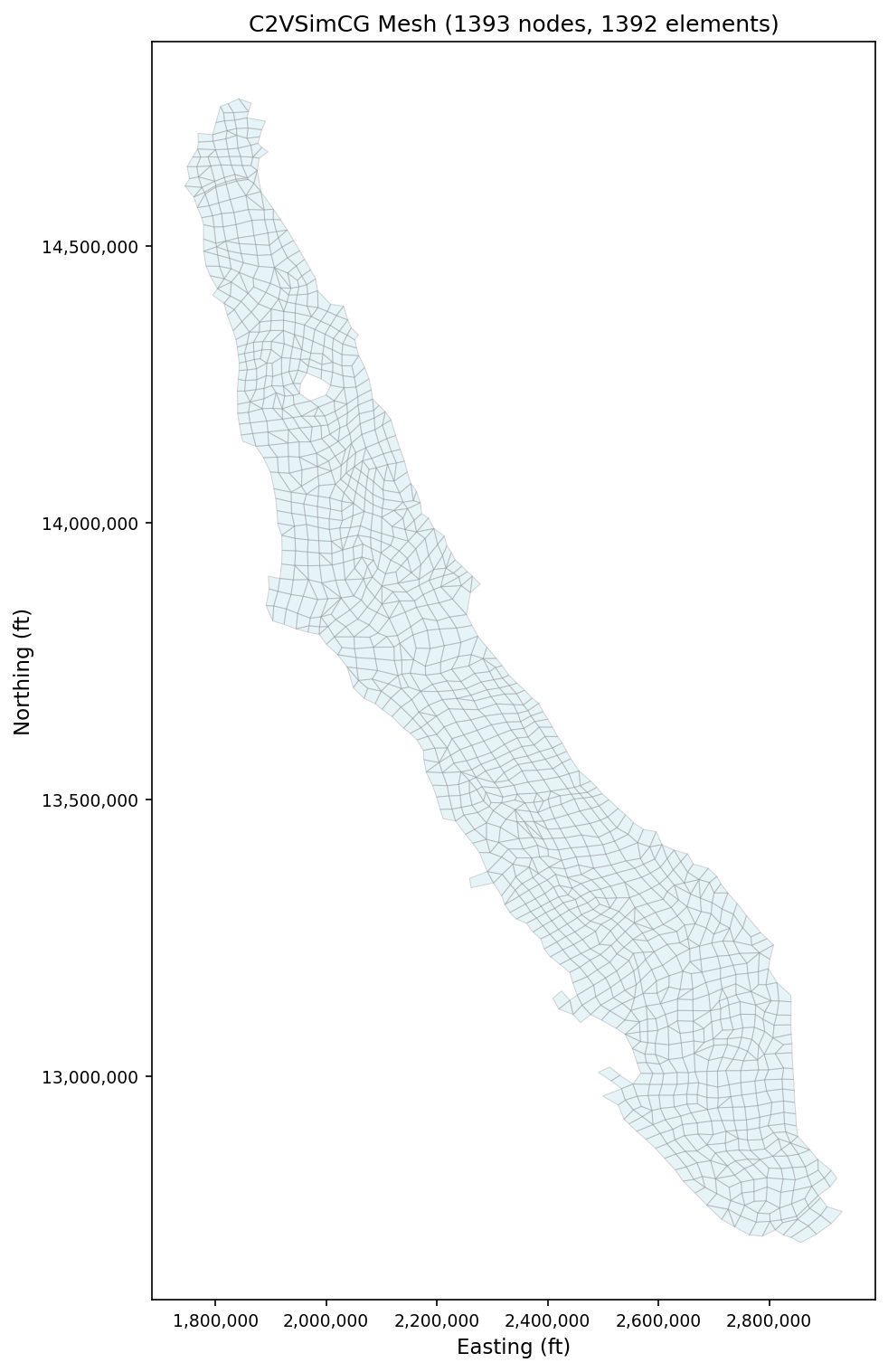
Visualize the mesh immediately after loading:

from pyiwfm.visualization.plotting import plot_mesh

fig, ax = plot_mesh(model.mesh, show_edges=True, edge_color='gray',
                    fill_color='lightblue', alpha=0.3, figsize=(10, 10))
ax.set_title(f'C2VSimCG Mesh ({model.n_nodes} nodes, {model.n_elements} elements)')
ax.set_xlabel('Easting (ft)')
ax.set_ylabel('Northing (ft)')

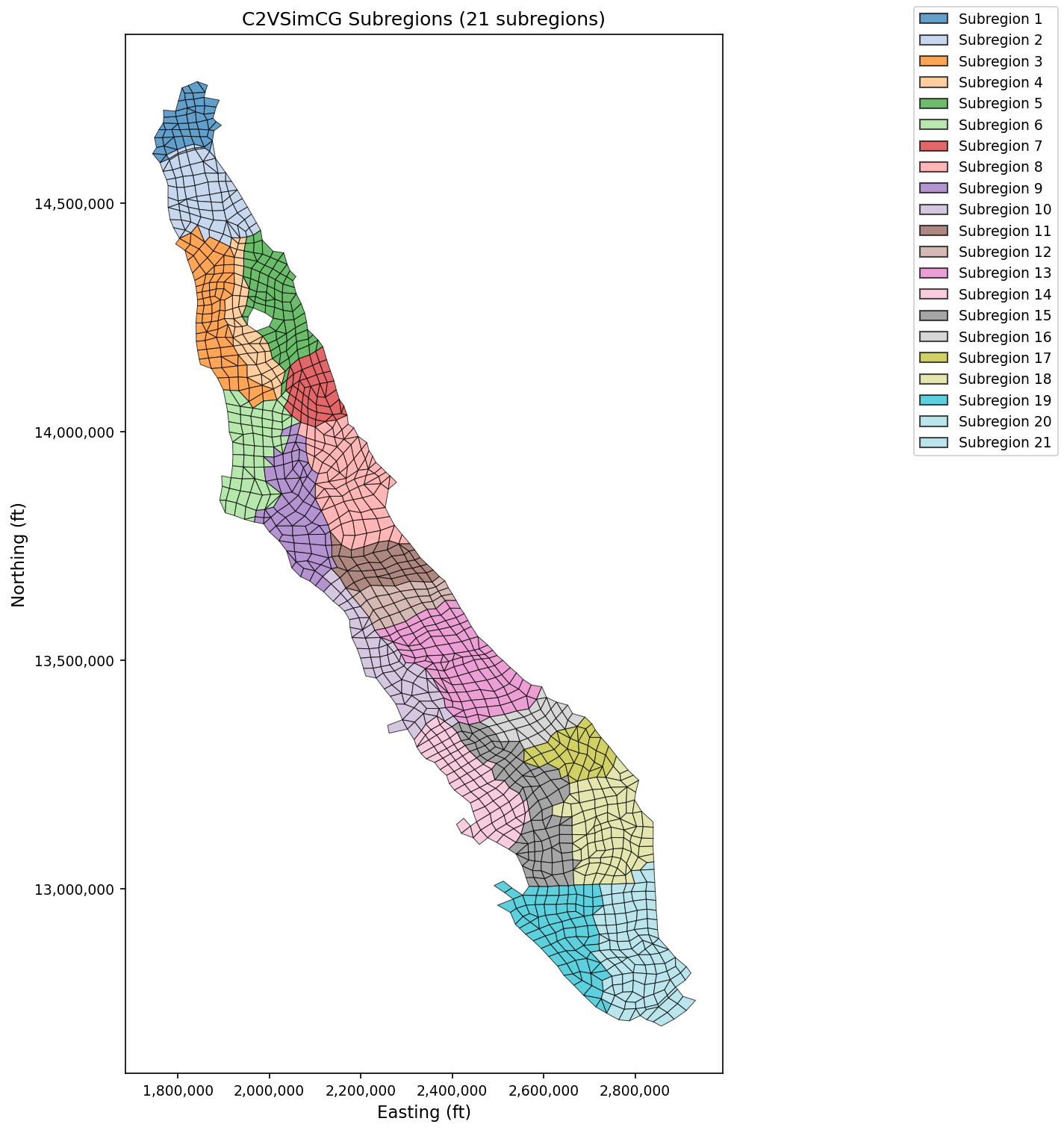
Color elements by subregion to see how the Central Valley is partitioned:

from pyiwfm.visualization.plotting import plot_elements

fig, ax = plot_elements(model.mesh, color_by='subregion',
                        cmap='Set3', alpha=0.7, figsize=(10, 10))
ax.set_title(f'C2VSimCG Subregions ({model.mesh.n_subregions} subregions)')

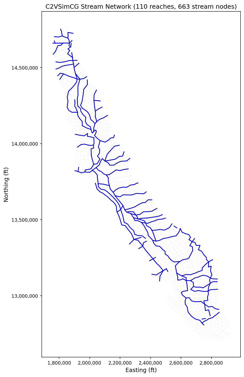
Stream Network#

Access the stream component to inspect reaches, stream nodes, diversions, and bypasses:

streams = model.streams
print(f"Stream Nodes: {streams.n_nodes}")
print(f"Reaches:      {streams.n_reaches}")
print(f"Diversions:   {streams.n_diversions}")
print(f"Bypasses:     {streams.n_bypasses}")

Overlay the stream network on the mesh:

from pyiwfm.visualization.plotting import plot_mesh, plot_streams

fig, ax = plot_mesh(model.mesh, show_edges=True, edge_color='lightgray',
                    fill_color='white', alpha=0.15, figsize=(10, 10))
plot_streams(model.streams, ax=ax, line_color='blue', line_width=1.5)
ax.set_title('C2VSimCG Stream Network')

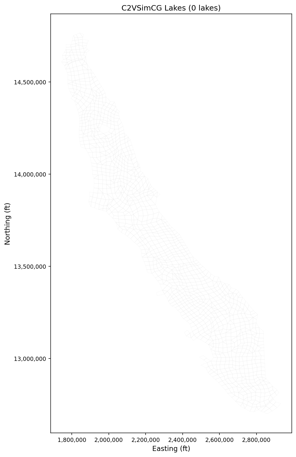
C2VSimCG stream network overlaid on mesh

Lakes#

Access the lake component:

lakes = model.lakes
print(f"Number of lakes: {lakes.n_lakes}")
print(f"Lake elements:   {lakes.n_lake_elements}")

Visualize lake boundaries on the mesh:

from pyiwfm.visualization.plotting import plot_lakes, plot_mesh

fig, ax = plot_mesh(model.mesh, show_edges=True, edge_color='lightgray',
                    fill_color='white', alpha=0.15, figsize=(10, 10))
plot_lakes(model.lakes, model.mesh, ax=ax, fill_color='cyan',
           edge_color='blue', alpha=0.5)
ax.set_title('C2VSimCG Lakes')

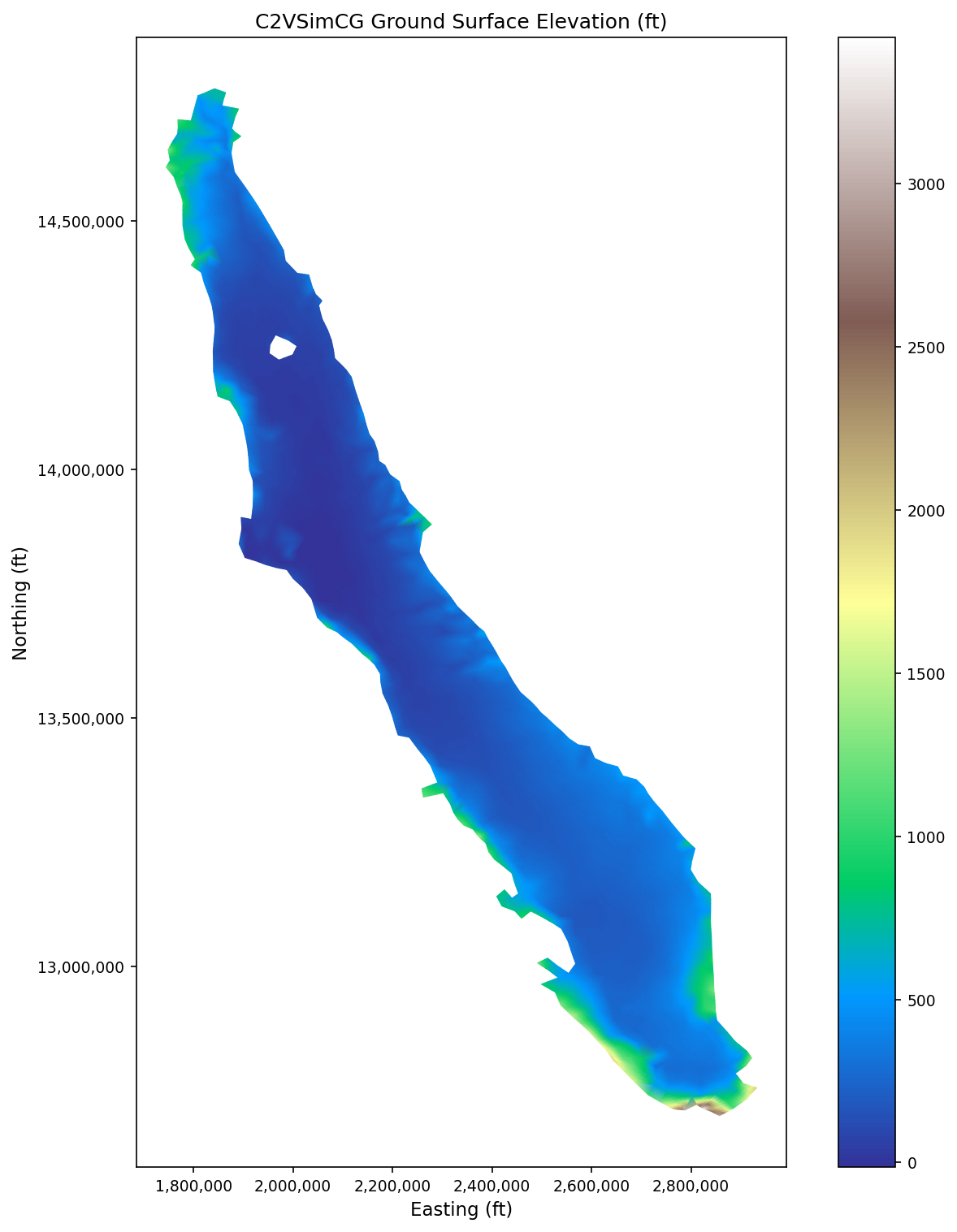
Stratigraphy and Ground Surface#

The stratigraphy contains ground surface elevation and layer top/bottom elevations at every node:

strat = model.stratigraphy
print(f"Layers:          {strat.n_layers}")
print(f"Nodes:           {strat.n_nodes}")
print(f"GS elev range:   {strat.gs_elev.min():.0f} - {strat.gs_elev.max():.0f} ft")

Plot the ground surface elevation as a scalar field:

from pyiwfm.visualization.plotting import plot_scalar_field

fig, ax = plot_scalar_field(model.mesh, strat.gs_elev,
                            field_type='node', cmap='terrain',
                            show_mesh=False, figsize=(10, 10))
ax.set_title('C2VSimCG Ground Surface Elevation (ft)')

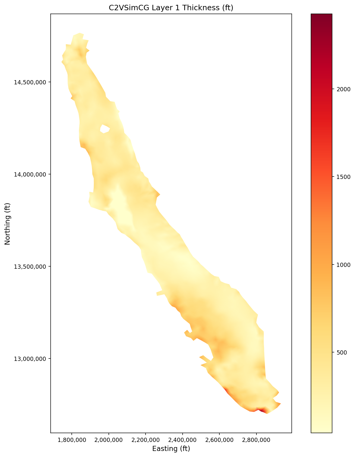
Compute and plot Layer 1 thickness:

thickness = strat.get_layer_thickness(0)  # Layer 1 (0-indexed)
fig, ax = plot_scalar_field(model.mesh, thickness,
                            field_type='node', cmap='YlOrRd',
                            show_mesh=False, figsize=(10, 10))
ax.set_title('C2VSimCG Layer 1 Thickness (ft)')

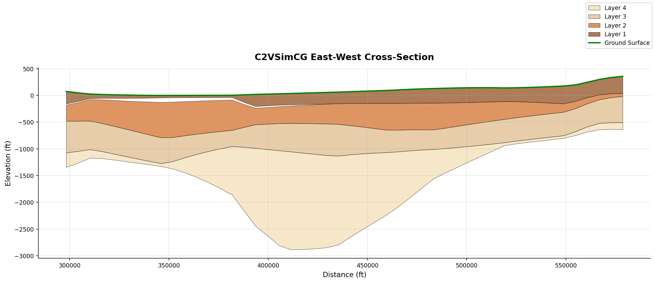
Extract and plot a vertical cross-section that cuts east-west through the center of the model domain:

from pyiwfm.core.cross_section import CrossSectionExtractor
from pyiwfm.visualization.plotting import plot_cross_section

extractor = CrossSectionExtractor(model.mesh, model.stratigraphy)
xs = extractor.extract(
    start=(x_min, y_mid),   # western edge, midpoint latitude
    end=(x_max, y_mid),     # eastern edge
    n_samples=200,
)
fig, ax = plot_cross_section(xs, title='C2VSimCG East-West Cross-Section')

C2VSimCG east-west stratigraphic cross-section

Loading with Error Handling#

For production code, use CompleteModelLoader which provides detailed diagnostics via ModelLoadResult:

from pyiwfm.io import CompleteModelLoader

loader = CompleteModelLoader(
    simulation_file="C2VSimCG/Simulation/Simulation.in",
    preprocessor_file="C2VSimCG/Preprocessor/Preprocessor.in",
)
result = loader.load()

# Check overall success
print(f"Success: {result.success}")

# Check for component-level errors
if result.has_errors:
    print("Component errors:")
    for component, error_msg in result.errors.items():
        print(f"  {component}: {error_msg}")

# Check warnings
if result.warnings:
    print("Warnings:")
    for warning in result.warnings:
        print(f"  - {warning}")

# Use the model (may have partial data if some components failed)
if result.model is not None:
    model = result.model
    print(f"Loaded {model.n_nodes} nodes, {model.n_elements} elements")

The loader continues loading remaining components even if one fails, storing errors in result.errors rather than raising exceptions. This allows you to work with the parts of the model that loaded successfully.

Loading Individual Components#

You can also load individual components directly using reader classes. This is useful when you only need specific parts of a model:

from pyiwfm.io import read_nodes, read_elements, read_stratigraphy

# Load just the mesh
nodes = read_nodes("C2VSimCG/Preprocessor/Nodal.dat")
elements = read_elements("C2VSimCG/Preprocessor/Element.dat")

from pyiwfm.core.mesh import AppGrid
grid = AppGrid(nodes=nodes, elements=elements)
grid.compute_connectivity()

print(f"Loaded mesh: {grid.n_nodes} nodes, {grid.n_elements} elements")

# Load stratigraphy separately
stratigraphy = read_stratigraphy("C2VSimCG/Preprocessor/Stratigraphy.dat")
print(f"Stratigraphy: {stratigraphy.n_layers} layers")

Or load just the preprocessor portion (mesh + stratigraphy + stream/lake geometry):

from pyiwfm.core.model import IWFMModel

model = IWFMModel.from_preprocessor("C2VSimCG/Preprocessor/Preprocessor.in")
print(f"Loaded mesh and stratigraphy only")
print(f"Nodes: {model.n_nodes}, Layers: {model.n_layers}")

Reading Simulation Results#

After running an IWFM simulation, load results for visualization:

Head data from output files:

from pyiwfm.io.hydrograph_reader import IWFMHydrographReader

# Read head hydrograph output
times, heads = read_hydrograph_file("C2VSimCG/Results/GW_Heads.out")
print(f"Head data: {len(times)} timesteps")

Budget data:

from pyiwfm.io import BudgetReader

reader = BudgetReader("C2VSimCG/Results/GW_Budget.hdf")
budget_data = reader.read()
print(f"Budget components: {list(budget_data.keys())}")

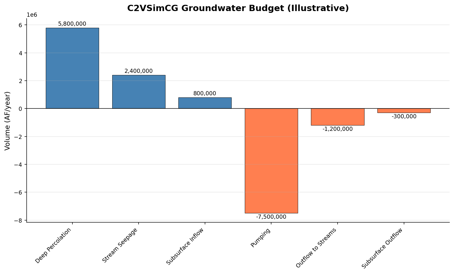
Read budget data directly from C2VSimCG’s HDF5 output files and visualize:

Budget bar chart (time-averaged):

from pyiwfm.io import BudgetReader
from pyiwfm.visualization.plotting import plot_budget_bar

reader = BudgetReader("C2VSimCG/Results/GW_Budget.hdf")

# Read the first location (whole-model summary) as a DataFrame
df = reader.get_dataframe(
    0,
    volume_factor=2.29568e-05,   # Cubic feet -> acre-feet
)

# Compute time-averaged budget components
budget_components = df.drop(columns=["Time"], errors="ignore").mean().to_dict()
print(f"Budget components: {list(budget_components.keys())}")

fig, ax = plot_budget_bar(budget_components,
                           title='C2VSimCG Groundwater Budget',
                           units='AF/month')

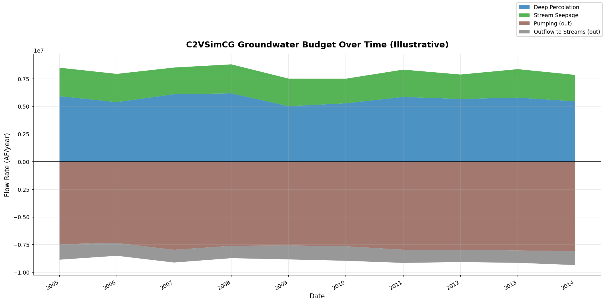
Budget stacked over time:

from pyiwfm.visualization.plotting import plot_budget_stacked

# Use the same DataFrame -- extract times and component columns
times = df["Time"].values
components = {
    col: df[col].values
    for col in df.columns if col != "Time"
}

fig, ax = plot_budget_stacked(times, components,
                               title='C2VSimCG GW Budget Over Time',
                               units='AF/month')

Comment-Preserving Load#

When you need to modify an IWFM model and write it back with all original comments intact, use the comment-preserving workflow:

from pyiwfm.io import load_model_with_comments

# Load model AND comment metadata
model, comments = load_model_with_comments("C2VSimCG/Simulation/Simulation.in")

# Inspect preserved comments
for file_key, metadata in comments.items():
    n_header = len(metadata.header_block) if metadata.header_block else 0
    n_sections = len(metadata.sections)
    print(f"  {file_key}: {n_header} header lines, {n_sections} sections")

# Make modifications to the model...
# model.groundwater.wells[5].pumping_rate *= 1.2

# Write back with preserved comments
from pyiwfm.io import save_complete_model
save_complete_model(model, "output_modified/")

This ensures that user comments, header blocks, and inline descriptions from the original files are retained in the output.

Exporting the Loaded Model#

Export to GIS formats for use in QGIS/ArcGIS:

from pyiwfm.visualization import GISExporter

exporter = GISExporter(
    grid=model.mesh,
    stratigraphy=model.stratigraphy,
    crs="EPSG:26910",  # NAD83 / UTM zone 10N
)

# Export to GeoPackage (nodes + elements + boundary)
exporter.export_geopackage("model_export.gpkg")
print("Exported to GeoPackage")

# Export to shapefiles
exporter.export_shapefiles("shapefiles/")

Export to VTK for 3D visualization in ParaView:

from pyiwfm.visualization import VTKExporter

vtk_exporter = VTKExporter(grid=model.mesh, stratigraphy=model.stratigraphy)

# 2D surface mesh
vtk_exporter.export_vtu("mesh_2d.vtu", mode="2d")

# Full 3D volumetric mesh
vtk_exporter.export_vtu("mesh_3d.vtu", mode="3d")

# With scalar data attached
vtk_exporter.export_vtu("mesh_with_heads.vtu", mode="3d",
                         node_scalars={"head": head_values})

For interactive visualization, launch the web viewer from the command line:

pyiwfm viewer --model-dir C2VSimCG/

Complete Script#

Here is a complete example combining all the steps above:

"""Load C2VSimCG, inspect it, and create visualizations."""

from pathlib import Path
from pyiwfm.io import CompleteModelLoader
from pyiwfm.core.cross_section import CrossSectionExtractor
from pyiwfm.visualization.plotting import (
    plot_mesh, plot_elements, plot_scalar_field,
    plot_streams, plot_lakes, plot_cross_section,
    plot_budget_bar,
)
from pyiwfm.visualization import GISExporter
import numpy as np

# --- Load the model ---
loader = CompleteModelLoader(
    simulation_file="C2VSimCG/Simulation/Simulation.in",
    preprocessor_file="C2VSimCG/Preprocessor/Preprocessor.in",
)
result = loader.load()

if not result.success:
    print(f"Load failed: {result.errors}")
    raise SystemExit(1)

model = result.model
print(model.summary())

# Print any warnings
for w in result.warnings:
    print(f"Warning: {w}")

# --- Output directory ---
output = Path("output_plots")
output.mkdir(exist_ok=True)

# --- Mesh ---
fig, ax = plot_mesh(model.mesh, show_edges=True, edge_color='gray', alpha=0.3)
ax.set_title(f'C2VSimCG Mesh ({model.n_nodes} nodes)')
fig.savefig(output / "mesh.png", dpi=150)

# --- Subregions ---
fig, ax = plot_elements(model.mesh, color_by='subregion', cmap='Set3')
ax.set_title(f'Subregions ({model.mesh.n_subregions})')
fig.savefig(output / "subregions.png", dpi=150)

# --- Ground surface elevation ---
fig, ax = plot_scalar_field(model.mesh, model.stratigraphy.gs_elev,
                            cmap='terrain', show_mesh=False)
ax.set_title('Ground Surface Elevation (ft)')
fig.savefig(output / "ground_surface.png", dpi=150)

# --- Layer 1 thickness ---
thickness = model.stratigraphy.get_layer_thickness(0)
fig, ax = plot_scalar_field(model.mesh, thickness, cmap='YlOrRd')
ax.set_title('Layer 1 Thickness (ft)')
fig.savefig(output / "layer1_thickness.png", dpi=150)

# --- Streams ---
if model.streams:
    fig, ax = plot_mesh(model.mesh, edge_color='lightgray', alpha=0.15)
    plot_streams(model.streams, ax=ax, line_width=1.5)
    ax.set_title('Stream Network')
    fig.savefig(output / "streams.png", dpi=150)

# --- Lakes ---
if model.lakes:
    fig, ax = plot_mesh(model.mesh, edge_color='lightgray', alpha=0.15)
    plot_lakes(model.lakes, model.mesh, ax=ax)
    ax.set_title('Lakes')
    fig.savefig(output / "lakes.png", dpi=150)

# --- Cross-section ---
all_x = [n.x for n in model.mesh.nodes.values()]
all_y = [n.y for n in model.mesh.nodes.values()]
extractor = CrossSectionExtractor(model.mesh, model.stratigraphy)
xs = extractor.extract(
    start=(min(all_x), (min(all_y) + max(all_y)) / 2),
    end=(max(all_x), (min(all_y) + max(all_y)) / 2),
    n_samples=200,
)
fig, ax = plot_cross_section(xs, title='East-West Cross-Section')
fig.savefig(output / "cross_section.png", dpi=150)

# --- Export to GIS ---
exporter = GISExporter(grid=model.mesh, crs="EPSG:26910")
exporter.export_geopackage(output / "model.gpkg")

print(f"All outputs saved to {output}/")

Next Steps#

See Tutorial: Building the IWFM Sample Model from Scratch for constructing a model from scratch
See Tutorial: Visualization for advanced plotting techniques
See Reading and Writing Files for all supported file formats
Launch the web viewer with pyiwfm viewer --model-dir C2VSimCG/