Tutorial: Mesh Generation#
This tutorial demonstrates how to create a finite element mesh for an IWFM model, starting from a boundary polygon and adding constraints for streams and wells.
Learning Objectives#
By the end of this tutorial, you will be able to:
Define a model boundary from coordinates
Add stream network constraints
Add well location constraints
Create refinement zones
Generate a triangular mesh
Export the mesh to GIS formats
Step 1: Import Libraries#
import numpy as np
from pathlib import Path

from pyiwfm.core.mesh import AppGrid, Node, Element
from pyiwfm.mesh_generation import TriangleMeshGenerator
from pyiwfm.mesh_generation.constraints import (
    Boundary,
    StreamConstraint,
    PointConstraint,
    RefinementZone,
)
from pyiwfm.visualization import GISExporter
from pyiwfm.visualization.plotting import plot_mesh
Step 2: Define the Model Boundary#
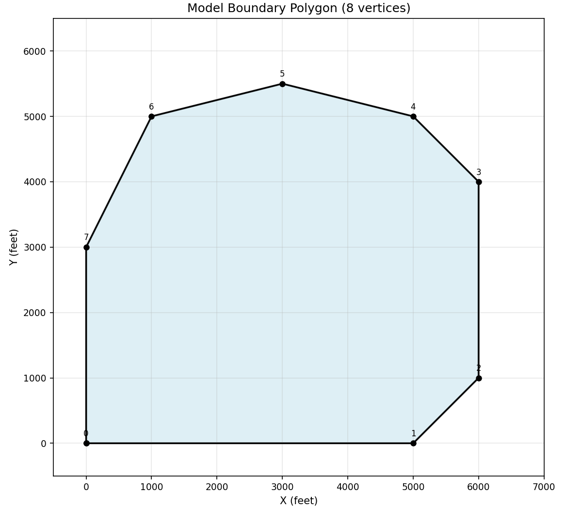
Define the boundary of your model domain. This can come from a shapefile or be defined manually with coordinates.
# Define an irregular polygon boundary (coordinates in feet)
boundary_coords = np.array([
    [0.0, 0.0],
    [5000.0, 0.0],
    [6000.0, 1000.0],
    [6000.0, 4000.0],
    [5000.0, 5000.0],
    [3000.0, 5500.0],
    [1000.0, 5000.0],
    [0.0, 3000.0],
])

# Create boundary
boundary = Boundary(vertices=boundary_coords)

print(f"Boundary has {boundary.n_vertices} vertices")
print(f"Approximate area: {boundary.area:.0f} sq ft")
Visualize the boundary polygon:
import numpy as np
import matplotlib.pyplot as plt
from matplotlib.patches import Polygon

boundary_coords = np.array([
    [0.0, 0.0], [5000.0, 0.0], [6000.0, 1000.0], [6000.0, 4000.0],
    [5000.0, 5000.0], [3000.0, 5500.0], [1000.0, 5000.0], [0.0, 3000.0],
])

fig, ax = plt.subplots(figsize=(8, 7))
poly = Polygon(boundary_coords, closed=True, fill=True,
                facecolor='lightblue', edgecolor='black', linewidth=2, alpha=0.4)
ax.add_patch(poly)
ax.plot(*np.vstack([boundary_coords, boundary_coords[0]]).T, 'ko-', markersize=5)
for i, (x, y) in enumerate(boundary_coords):
    ax.annotate(f'{i}', (x, y), fontsize=8, ha='center', va='bottom',
                xytext=(0, 5), textcoords='offset points')
ax.set_xlim(-500, 7000)
ax.set_ylim(-500, 6500)
ax.set_aspect('equal')
ax.set_xlabel('X (feet)')
ax.set_ylabel('Y (feet)')
ax.set_title('Model Boundary Polygon (8 vertices)')
ax.grid(True, alpha=0.3)
plt.show()
Step 3: Add Stream Constraints#
Define stream reaches that must be honored by the mesh. The mesh generator will place nodes along the stream and create elements that follow the stream.
# Main river (flows from NE to SW)
river_coords = np.array([
    [5500.0, 4500.0],  # Upstream
    [4000.0, 3500.0],
    [3000.0, 3000.0],
    [2000.0, 2000.0],
    [500.0, 1000.0],   # Downstream
])
river = StreamConstraint(vertices=river_coords, stream_id=1)

# Tributary (joins main river)
tributary_coords = np.array([
    [4500.0, 1000.0],  # Upstream
    [3500.0, 1500.0],
    [2000.0, 2000.0],  # Confluence
])
tributary = StreamConstraint(vertices=tributary_coords, stream_id=2)

stream_constraints = [river, tributary]
print(f"Added {len(stream_constraints)} stream constraints")
Step 4: Add Well Locations#
Add point constraints for well locations. The mesh generator will ensure nodes exist at these exact locations.
# Define well locations
well_locations = [
    (1500.0, 3500.0, "Well-1"),
    (3500.0, 4000.0, "Well-2"),
    (4500.0, 2500.0, "Well-3"),
    (2000.0, 1000.0, "Well-4"),
]

well_constraints = [
    PointConstraint(x=x, y=y)
    for x, y, _name in well_locations
]

print(f"Added {len(well_constraints)} well locations")
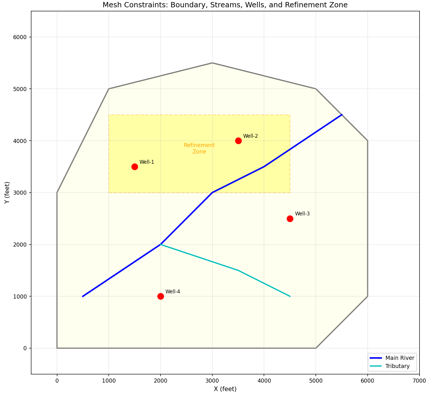
Visualize all constraints together before mesh generation:
import numpy as np
import matplotlib.pyplot as plt
from matplotlib.patches import Polygon

boundary_coords = np.array([
    [0.0, 0.0], [5000.0, 0.0], [6000.0, 1000.0], [6000.0, 4000.0],
    [5000.0, 5000.0], [3000.0, 5500.0], [1000.0, 5000.0], [0.0, 3000.0],
])
river_coords = np.array([
    [5500.0, 4500.0], [4000.0, 3500.0], [3000.0, 3000.0],
    [2000.0, 2000.0], [500.0, 1000.0],
])
tributary_coords = np.array([
    [4500.0, 1000.0], [3500.0, 1500.0], [2000.0, 2000.0],
])
wells = [(1500.0, 3500.0, "Well-1"), (3500.0, 4000.0, "Well-2"),
         (4500.0, 2500.0, "Well-3"), (2000.0, 1000.0, "Well-4")]
refine_north = np.array([
    [1000.0, 3000.0], [4500.0, 3000.0], [4500.0, 4500.0], [1000.0, 4500.0],
])

fig, ax = plt.subplots(figsize=(10, 9))
poly = Polygon(boundary_coords, closed=True, fill=True,
                facecolor='lightyellow', edgecolor='black', linewidth=2, alpha=0.5)
ax.add_patch(poly)
ax.plot(river_coords[:, 0], river_coords[:, 1], 'b-', linewidth=2.5, label='Main River')
ax.plot(tributary_coords[:, 0], tributary_coords[:, 1], 'c-', linewidth=2, label='Tributary')
refine_poly = Polygon(refine_north, closed=True, fill=True,
                       facecolor='yellow', edgecolor='orange', linewidth=1.5,
                       alpha=0.3, linestyle='--')
ax.add_patch(refine_poly)
ax.text(2750, 3750, 'Refinement\nZone', ha='center', fontsize=9, color='orange')
for x, y, name in wells:
    ax.plot(x, y, 'ro', markersize=10, zorder=5)
    ax.annotate(name, (x, y), xytext=(8, 5), textcoords='offset points', fontsize=8)
ax.set_xlim(-500, 7000)
ax.set_ylim(-500, 6500)
ax.set_aspect('equal')
ax.set_xlabel('X (feet)')
ax.set_ylabel('Y (feet)')
ax.set_title('Mesh Constraints: Boundary, Streams, Wells, and Refinement Zone')
ax.legend(loc='lower right')
ax.grid(True, alpha=0.3)
plt.show()
Step 5: Define Refinement Zones#
Create areas where you want finer mesh resolution, such as near pumping wells or in areas of interest.
# Refinement zone around wells 1 and 2 (northern area)
refine_north = RefinementZone(
    polygon=np.array([
        [1000.0, 3000.0],
        [4500.0, 3000.0],
        [4500.0, 4500.0],
        [1000.0, 4500.0],
    ]),
    max_area=10000.0,  # Smaller elements
)

# Refinement zone along main river corridor
refine_river = RefinementZone(
    polygon=np.array([
        [500.0, 500.0],
        [4500.0, 2500.0],
        [4000.0, 4000.0],
        [1500.0, 3500.0],
        [0.0, 2500.0],
    ]),
    max_area=15000.0,
)

refinement_zones = [refine_north, refine_river]
print(f"Added {len(refinement_zones)} refinement zones")
Step 6: Generate the Mesh#
Use the Triangle mesh generator to create the mesh.
# Create mesh generator
generator = TriangleMeshGenerator()

# Generate mesh with all constraints
result = generator.generate(
    boundary=boundary,
    streams=stream_constraints,
    points=well_constraints,
    refinement_zones=refinement_zones,
    max_area=50000.0,    # Maximum element area (coarse areas)
    min_angle=25.0,      # Minimum angle for quality
)

print(f"Generated mesh:")
print(f"  Nodes: {result.n_nodes}")
print(f"  Elements: {result.n_elements}")
Step 7: Convert to AppGrid#
Convert the mesh result to an AppGrid for use with other pyiwfm modules.
# Convert to AppGrid
grid = result.to_appgrid()

# Verify the conversion
print(f"AppGrid created:")
print(f"  Nodes: {grid.n_nodes}")
print(f"  Elements: {grid.n_elements}")
print(f"  Boundary nodes: {grid.n_boundary_nodes}")
Step 8: Visualize the Mesh#
Plot the mesh to verify it looks correct.
# Create mesh plot
fig, ax = plot_mesh(
    grid,
    show_edges=True,
    edge_color="gray",
    fill_color="lightblue",
    alpha=0.3,
    figsize=(12, 10),
)

# Add stream lines to the plot
for stream in stream_constraints:
    ax.plot(stream.vertices[:, 0], stream.vertices[:, 1],
            'b-', linewidth=2, label=f"Stream {stream.stream_id}")

# Add well locations
for x, y, name in well_locations:
    ax.plot(x, y, 'ro', markersize=8)
    ax.annotate(name, (x, y), xytext=(5, 5), textcoords='offset points')

ax.set_title("Generated Finite Element Mesh")
ax.legend()
fig.savefig("mesh_with_constraints.png", dpi=150, bbox_inches="tight")
print("Saved mesh plot to mesh_with_constraints.png")
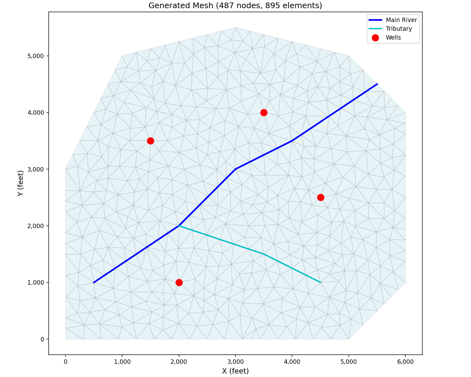
Here is the actual mesh produced by the Triangle generator with the constraints defined above:
import numpy as np
import matplotlib.pyplot as plt
from pyiwfm.mesh_generation import TriangleMeshGenerator
from pyiwfm.mesh_generation.constraints import (
    Boundary, StreamConstraint, PointConstraint, RefinementZone,
)
from pyiwfm.visualization.plotting import plot_mesh

boundary = Boundary(vertices=np.array([
    [0, 0], [5000, 0], [6000, 1000], [6000, 4000],
    [5000, 5000], [3000, 5500], [1000, 5000], [0, 3000],
]))
river = StreamConstraint(vertices=np.array([
    [5500, 4500], [4000, 3500], [3000, 3000], [2000, 2000], [500, 1000],
]), stream_id=1)
tributary = StreamConstraint(vertices=np.array([
    [4500, 1000], [3500, 1500], [2000, 2000],
]), stream_id=2)
wells = [
    PointConstraint(x=1500, y=3500),
    PointConstraint(x=3500, y=4000),
    PointConstraint(x=4500, y=2500),
    PointConstraint(x=2000, y=1000),
]
refine_north = RefinementZone(
    polygon=np.array([[1000, 3000], [4500, 3000], [4500, 4500], [1000, 4500]]),
    max_area=10000.0,
)
refine_river = RefinementZone(
    polygon=np.array([
        [500, 500], [4500, 2500], [4000, 4000], [1500, 3500], [0, 2500],
    ]),
    max_area=15000.0,
)

generator = TriangleMeshGenerator()
result = generator.generate(
    boundary=boundary,
    streams=[river, tributary],
    points=wells,
    refinement_zones=[refine_north, refine_river],
    max_area=50000.0, min_angle=25.0,
)
grid = result.to_appgrid()

fig, ax = plot_mesh(grid, show_edges=True, edge_color='gray',
                    fill_color='lightblue', alpha=0.3, figsize=(10, 8))
ax.plot([5500, 4000, 3000, 2000, 500], [4500, 3500, 3000, 2000, 1000],
        'b-', linewidth=2.5, label='Main River')
ax.plot([4500, 3500, 2000], [1000, 1500, 2000],
        'c-', linewidth=2, label='Tributary')
for pc in wells:
    ax.plot(pc.x, pc.y, 'ro', markersize=10, zorder=5)
ax.plot([], [], 'ro', markersize=10, label='Wells')
ax.set_title(f'Generated Mesh ({grid.n_nodes} nodes, {grid.n_elements} elements)')
ax.set_xlabel('X (feet)')
ax.set_ylabel('Y (feet)')
ax.legend()
plt.show()
Step 9: Export to GIS#
Export the mesh to a GeoPackage for use in GIS software.
# Create GIS exporter with coordinate reference system
exporter = GISExporter(
    grid=grid,
    crs="EPSG:2227",  # NAD83 / California Zone 3 (feet)
)

# Export to GeoPackage
output_dir = Path("output")
output_dir.mkdir(exist_ok=True)

exporter.export_geopackage(
    output_dir / "model_mesh.gpkg",
    include_boundary=True,
)
print(f"Exported mesh to {output_dir / 'model_mesh.gpkg'}")

# Also export as shapefiles
exporter.export_shapefiles(output_dir / "shapefiles")
print(f"Exported shapefiles to {output_dir / 'shapefiles'}")
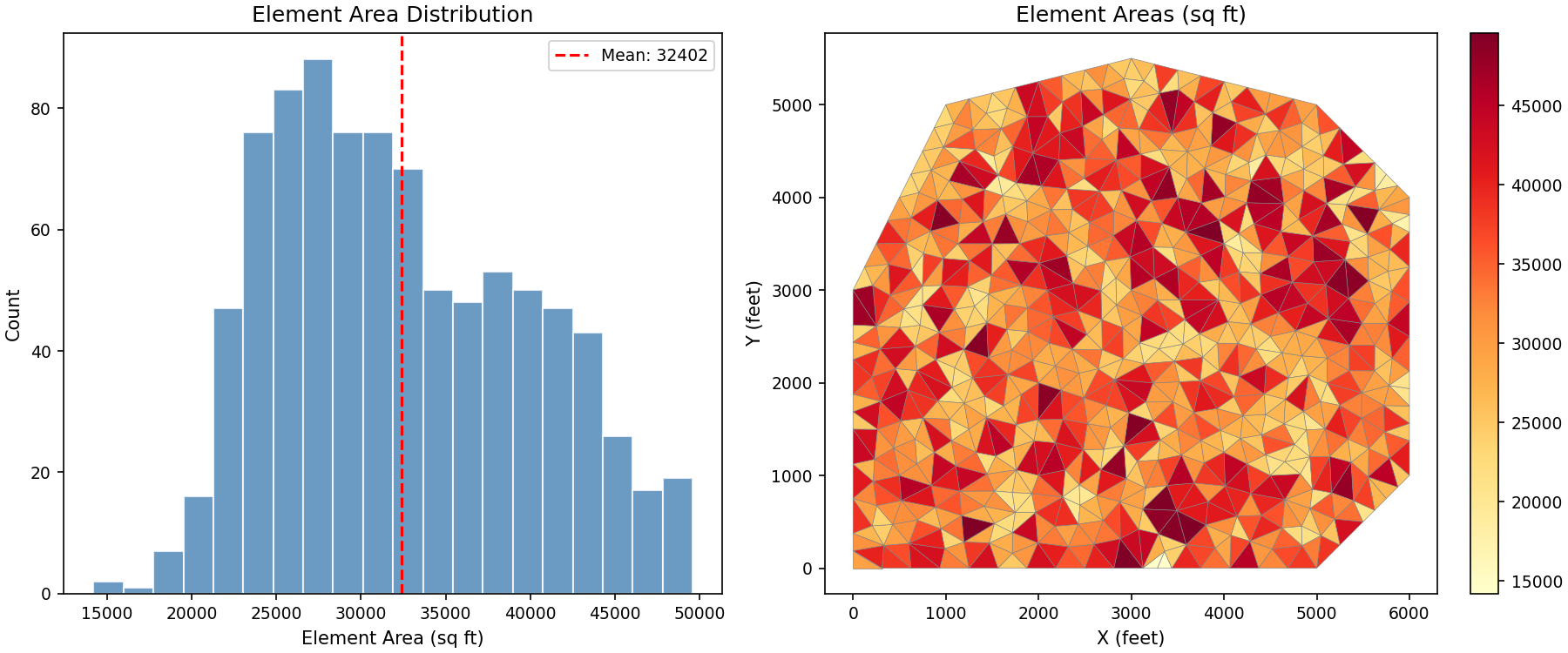
Step 10: Analyze Mesh Quality#
Check the quality of the generated mesh.
# Calculate element areas
areas = []
for elem in grid.iter_elements():
    coords = np.array([
        [grid.nodes[v].x, grid.nodes[v].y]
        for v in elem.vertices
    ])
    n = len(coords)
    area = 0.5 * abs(sum(
        coords[i, 0] * coords[(i + 1) % n, 1] -
        coords[(i + 1) % n, 0] * coords[i, 1]
        for i in range(n)
    ))
    areas.append(area)

areas = np.array(areas)

print("Mesh Quality Statistics:")
print(f"  Total elements: {len(areas)}")
print(f"  Minimum area: {areas.min():.1f} sq ft")
print(f"  Maximum area: {areas.max():.1f} sq ft")
print(f"  Mean area: {areas.mean():.1f} sq ft")
print(f"  Median area: {np.median(areas):.1f} sq ft")
print(f"  Area ratio (max/min): {areas.max() / areas.min():.1f}")
Visualize the element area distribution:
import numpy as np
import matplotlib.pyplot as plt
from matplotlib.collections import PolyCollection
from pyiwfm.mesh_generation import TriangleMeshGenerator
from pyiwfm.mesh_generation.constraints import (
    Boundary, StreamConstraint, PointConstraint, RefinementZone,
)

boundary = Boundary(vertices=np.array([
    [0, 0], [5000, 0], [6000, 1000], [6000, 4000],
    [5000, 5000], [3000, 5500], [1000, 5000], [0, 3000],
]))
river = StreamConstraint(vertices=np.array([
    [5500, 4500], [4000, 3500], [3000, 3000], [2000, 2000], [500, 1000],
]))
tributary = StreamConstraint(vertices=np.array([
    [4500, 1000], [3500, 1500], [2000, 2000],
]))
wells = [
    PointConstraint(x=1500, y=3500), PointConstraint(x=3500, y=4000),
    PointConstraint(x=4500, y=2500), PointConstraint(x=2000, y=1000),
]
refine_north = RefinementZone(
    polygon=np.array([[1000, 3000], [4500, 3000], [4500, 4500], [1000, 4500]]),
    max_area=10000.0,
)
refine_river = RefinementZone(
    polygon=np.array([
        [500, 500], [4500, 2500], [4000, 4000], [1500, 3500], [0, 2500],
    ]),
    max_area=15000.0,
)

generator = TriangleMeshGenerator()
result = generator.generate(
    boundary=boundary,
    streams=[river, tributary],
    points=wells,
    refinement_zones=[refine_north, refine_river],
    max_area=50000.0, min_angle=25.0,
)
grid = result.to_appgrid()

# Compute element areas
areas = []
for elem in grid.elements.values():
    coords = np.array([[grid.nodes[v].x, grid.nodes[v].y] for v in elem.vertices])
    n = len(coords)
    area = 0.5 * abs(sum(
        coords[i, 0] * coords[(i + 1) % n, 1] -
        coords[(i + 1) % n, 0] * coords[i, 1]
        for i in range(n)))
    areas.append(area)
areas = np.array(areas)

fig, axes = plt.subplots(1, 2, figsize=(12, 5))

# Histogram
axes[0].hist(areas, bins=20, color='steelblue', edgecolor='white', alpha=0.8)
axes[0].axvline(areas.mean(), color='red', linestyle='--', label=f'Mean: {areas.mean():.0f}')
axes[0].set_xlabel('Element Area (sq ft)')
axes[0].set_ylabel('Count')
axes[0].set_title('Element Area Distribution')
axes[0].legend()

# Element areas as colored mesh
polys = []
for elem in grid.elements.values():
    coords = [(grid.nodes[v].x, grid.nodes[v].y) for v in elem.vertices]
    polys.append(coords)
pc = PolyCollection(polys, array=areas, cmap='YlOrRd', edgecolors='gray', linewidths=0.3)
axes[1].add_collection(pc)
axes[1].autoscale()
axes[1].set_aspect('equal')
axes[1].set_xlabel('X (feet)')
axes[1].set_ylabel('Y (feet)')
axes[1].set_title('Element Areas (sq ft)')
plt.colorbar(pc, ax=axes[1])

plt.show()
Complete Script#
Here’s the complete script combining all steps:
"""Complete mesh generation example."""

import numpy as np
from pathlib import Path

from pyiwfm.mesh_generation import TriangleMeshGenerator
from pyiwfm.mesh_generation.constraints import (
    Boundary, StreamConstraint, PointConstraint, RefinementZone
)
from pyiwfm.visualization import GISExporter
from pyiwfm.visualization.plotting import plot_mesh

# 1. Define boundary
boundary = Boundary(vertices=np.array([
    [0, 0], [5000, 0], [6000, 1000], [6000, 4000],
    [5000, 5000], [3000, 5500], [1000, 5000], [0, 3000]
]))

# 2. Define streams
river = StreamConstraint(vertices=np.array([
    [5500, 4500], [4000, 3500], [3000, 3000], [2000, 2000], [500, 1000]
]))

# 3. Define wells
wells = [PointConstraint(x=1500, y=3500), PointConstraint(x=3500, y=4000)]

# 4. Define refinement
refine = RefinementZone(
    polygon=np.array([[1000, 3000], [4500, 3000], [4500, 4500], [1000, 4500]]),
    max_area=10000
)

# 5. Generate mesh
generator = TriangleMeshGenerator()
result = generator.generate(
    boundary=boundary,
    streams=[river],
    points=wells,
    refinement_zones=[refine],
    max_area=50000,
    min_angle=25
)

# 6. Convert and export
grid = result.to_appgrid()
exporter = GISExporter(grid=grid, crs="EPSG:2227")
exporter.export_geopackage("model.gpkg")

print(f"Generated {grid.n_nodes} nodes, {grid.n_elements} elements")
Next Steps#
Add stratigraphy to create a complete 3D model
Export to VTK for 3D visualization in ParaView
Try the Gmsh generator for quadrilateral elements