Tutorial: Calibration Workflow#
This tutorial demonstrates pyiwfm’s calibration tools: reading SMP observation files, interpolating simulated heads to observation times, clustering wells, computing typical hydrographs, and creating publication-quality calibration figures.
Learning Objectives#
By the end of this tutorial, you will be able to:
Read and write SMP observation files
Interpolate simulated heads to observation timestamps (IWFM2OBS)
Auto-discover model files and run IWFM2OBS from a simulation main file
Cluster observation wells using fuzzy c-means
Compute typical hydrographs by cluster (CalcTypHyd)
Create 1:1 plots, residual histograms, and calibration summary figures
Parse SimulationMessages.out for spatial error diagnostics
Step 1: Reading SMP Files#
The SMP (Sample/Bore) format is IWFM’s standard observation file format. Each record contains a bore ID, date/time, value, and optional exclusion flag.
from pyiwfm.io.smp import SMPReader

# Read all bores from an SMP file
reader = SMPReader("observed_heads.smp")
observed = reader.read()

print(f"Loaded {len(observed)} bores")
for bore_id, ts in list(observed.items())[:3]:
    print(f"  {bore_id}: {len(ts.times)} records, "
          f"range {ts.values.min():.1f} - {ts.values.max():.1f}")
Read a single bore:
ts = reader.read_bore("WELL-001")
if ts is not None:
    print(f"Bore {ts.bore_id}: {len(ts.times)} records")
Write SMP data back to a file:
from pyiwfm.io.smp import SMPWriter

writer = SMPWriter("output.smp")
writer.write(observed)
Step 2: IWFM2OBS – Interpolate to Observation Times#
The interpolate_to_obs_times function linearly interpolates simulated
time series to match observation timestamps, mirroring the Fortran IWFM2OBS
utility:
from pyiwfm.calibration.iwfm2obs import (
    interpolate_to_obs_times,
    interpolate_batch,
    InterpolationConfig,
)

# Configure interpolation
config = InterpolationConfig(
    max_extrapolation_time=timedelta(days=30),
    sentinel_value=-999.0,
    interpolation_method="linear",
)

# Interpolate a single bore
interp_ts = interpolate_to_obs_times(
    observed=observed["WELL-001"],
    simulated=simulated["WELL-001"],
    config=config,
)
print(f"Interpolated {len(interp_ts.values)} values")

# Interpolate all matching bores at once
results = interpolate_batch(observed, simulated, config)
print(f"Interpolated {len(results)} bores")
For multi-layer observation wells that screen multiple aquifer layers, use transmissivity-weighted composite heads:
from pyiwfm.calibration.iwfm2obs import (
    MultiLayerWellSpec,
    compute_multilayer_weights,
    compute_composite_head,
)

well = MultiLayerWellSpec(
    name="DEEP-WELL-01",
    x=1_200_000.0,
    y=600_000.0,
    element_id=42,
    bottom_of_screen=-50.0,
    top_of_screen=20.0,
)

weights = compute_multilayer_weights(
    well, grid, stratigraphy, hydraulic_conductivity
)
print(f"Layer weights: {weights}")

composite = compute_composite_head(well, layer_heads, weights, grid)
print(f"Composite head: {composite:.2f} ft")
The full IWFM2OBS workflow reads SMP files, interpolates, and writes output:
from pyiwfm.calibration.iwfm2obs import iwfm2obs

results = iwfm2obs(
    obs_smp_path=Path("observed.smp"),
    sim_smp_path=Path("simulated.smp"),
    output_path=Path("interpolated.smp"),
)
print(f"Wrote {len(results)} interpolated bores")
Step 2b: Model-Discovery Mode (IWFM2OBS from Simulation Main File)#
Instead of working with pre-converted SMP files, you can point directly at
the IWFM simulation main file. pyiwfm will auto-discover the GW and stream
hydrograph .out files, read them, interpolate to observation times, and
optionally compute multi-layer T-weighted averages — all in one call.
Discover model files:
from pyiwfm.calibration.model_file_discovery import discover_hydrograph_files

info = discover_hydrograph_files("C2VSimFG.in")

print(f"GW .out file:     {info.gw_hydrograph_path}")
print(f"Stream .out file: {info.stream_hydrograph_path}")
print(f"GW locations:     {len(info.gw_locations)}")
print(f"Start date:       {info.start_date_str}")
print(f"Time unit:        {info.time_unit}")
Run the full workflow:
from pathlib import Path
from pyiwfm.calibration.iwfm2obs import iwfm2obs_from_model

results = iwfm2obs_from_model(
    simulation_main_file=Path("C2VSimFG.in"),
    obs_smp_paths={"gw": Path("GW_Obs.smp")},
    output_paths={"gw": Path("GW_OUT.smp")},
)

for hyd_type, bore_results in results.items():
    print(f"{hyd_type}: interpolated {len(bore_results)} bore(s)")
Multi-layer observation wells:
For wells that screen multiple aquifer layers, provide a well specification
file and output paths for the GW_MultiLayer.out and PEST .ins files:
from pyiwfm.calibration.obs_well_spec import read_obs_well_spec

well_specs = read_obs_well_spec("obs_wells.txt")
for w in well_specs[:3]:
    print(f"  {w.name}: elem={w.element_id}, "
          f"screen={w.top_of_screen:.0f} to {w.bottom_of_screen:.0f}")

results = iwfm2obs_from_model(
    simulation_main_file=Path("C2VSimFG.in"),
    obs_smp_paths={"gw": Path("GW_Obs.smp")},
    output_paths={"gw": Path("GW_OUT.smp")},
    obs_well_spec_path=Path("obs_wells.txt"),
    multilayer_output_path=Path("GW_MultiLayer.out"),
    multilayer_ins_path=Path("GWHMultiLayer.ins"),
)
Write multi-layer outputs manually:
from pyiwfm.calibration.iwfm2obs import (
    write_multilayer_output,
    write_multilayer_pest_ins,
)

# write_multilayer_output writes: Name, Date, Time, Simulated, T1-T4, NewTOS, NewBOS
write_multilayer_output(results_dict, well_specs, weights, Path("GW_MultiLayer.out"), n_layers=4)

# write_multilayer_pest_ins writes: pif #, l1, l1 [WLT00001_00001]50:60, ...
write_multilayer_pest_ins(results_dict, well_specs, Path("GWHMultiLayer.ins"))
CLI model-discovery mode:
# Auto-discover .out files and interpolate
pyiwfm iwfm2obs --model C2VSimFG.in --obs-gw GW_Obs.smp --output-gw GW_OUT.smp

# With multi-layer processing
pyiwfm iwfm2obs --model C2VSimFG.in \
    --obs-gw GW_Obs.smp --output-gw GW_OUT.smp \
    --well-spec obs_wells.txt \
    --multilayer-out GW_MultiLayer.out \
    --multilayer-ins GWHMultiLayer.ins
Step 3: Cluster Observation Wells#
Fuzzy c-means clustering groups wells by both spatial proximity and temporal behavior (amplitude, trend, seasonality):
from pyiwfm.calibration.clustering import (
    ClusteringConfig,
    fuzzy_cmeans_cluster,
)

# Well locations: dict[str, tuple[float, float]]
locations = {bore_id: (x, y) for bore_id, (x, y) in well_coords.items()}

config = ClusteringConfig(
    n_clusters=5,
    fuzziness=2.0,
    spatial_weight=0.3,
    temporal_weight=0.7,
    random_seed=42,
)

result = fuzzy_cmeans_cluster(locations, observed, config)

print(f"Clusters: {result.n_clusters}")
print(f"FPC (partition coefficient): {result.fpc:.3f}")
print(f"Membership matrix shape: {result.membership.shape}")

# Get the dominant cluster for a specific well
cluster_id = result.get_dominant_cluster("WELL-001")
print(f"WELL-001 is in cluster {cluster_id}")

# Get all wells in a cluster (membership > 0.5)
wells_in_c0 = result.get_cluster_wells(0, threshold=0.5)
print(f"Cluster 0 wells: {wells_in_c0}")
Export cluster weights for use with CalcTypHyd:
result.to_weights_file(Path("cluster_weights.txt"))
Step 4: Compute Typical Hydrographs (CalcTypHyd)#
Typical hydrographs represent the characteristic seasonal pattern for each cluster, computed by seasonal averaging, de-meaning, and membership-weighted combination:
from pyiwfm.calibration.calctyphyd import (
    CalcTypHydConfig,
    compute_typical_hydrographs,
    read_cluster_weights,
)

# Read cluster weights from file (or use result.membership directly)
cluster_weights = read_cluster_weights(Path("cluster_weights.txt"))

config = CalcTypHydConfig(
    min_records_per_season=1,
)

typ_result = compute_typical_hydrographs(
    water_levels=observed,
    cluster_weights=cluster_weights,
    config=config,
)

for th in typ_result.hydrographs:
    print(f"Cluster {th.cluster_id}: "
          f"{len(th.contributing_wells)} wells, "
          f"range {th.values[~np.isnan(th.values)].min():.2f} "
          f"to {th.values[~np.isnan(th.values)].max():.2f}")
Step 5: Calibration Metrics#
Compute performance metrics including the new Scaled RMSE (SRMSE):
from pyiwfm.comparison.metrics import ComparisonMetrics, scaled_rmse

# Compute all metrics at once
metrics = ComparisonMetrics.compute(obs_values, sim_values)
print(metrics.summary())
print(f"Scaled RMSE: {metrics.scaled_rmse:.4f}")

# Or compute SRMSE individually
srmse = scaled_rmse(obs_values, sim_values)
print(f"SRMSE = {srmse:.4f}")
Step 6: Calibration Plots#
Create publication-quality calibration figures using the dedicated
calibration_plots module. All functions use a publication matplotlib
style (serif fonts, no top/right spines, 300 DPI).
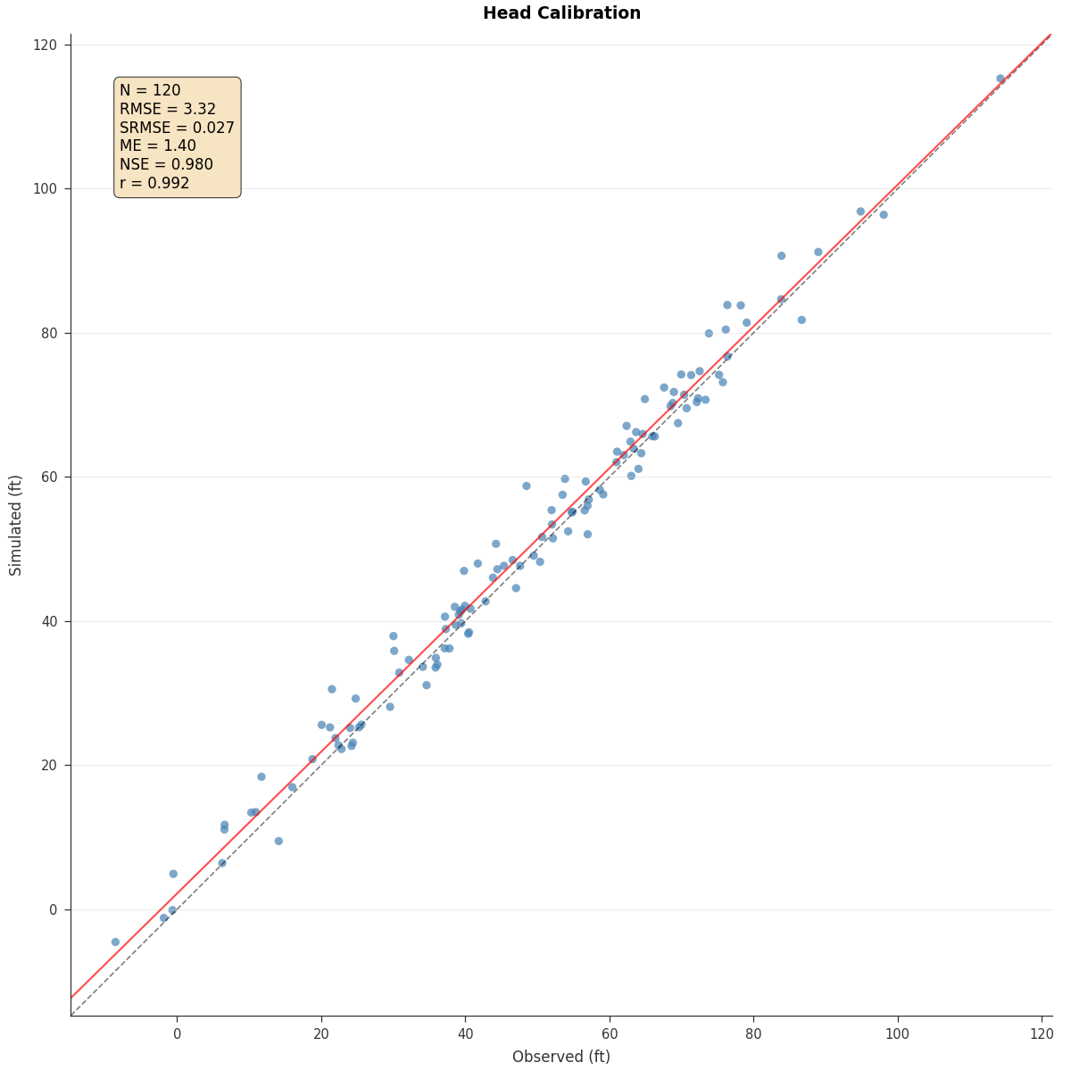
1:1 Plot (Observed vs Simulated):
from pyiwfm.visualization.plotting import plot_one_to_one

fig, ax = plot_one_to_one(
    obs_values, sim_values,
    show_metrics=True,
    show_identity=True,
    show_regression=True,
    title="Head Calibration",
    units="ft",
)
fig.savefig("one_to_one.png", dpi=300)
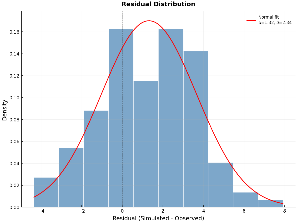
Residual Histogram:
from pyiwfm.visualization.calibration_plots import plot_residual_histogram

residuals = sim_values - obs_values
fig, ax = plot_residual_histogram(
    residuals,
    show_normal_fit=True,
)
fig.savefig("residual_hist.png", dpi=300)
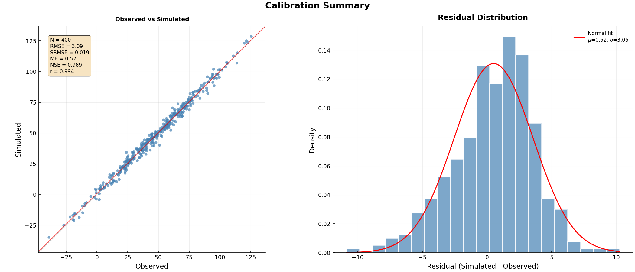
Multi-panel Calibration Summary:
from pyiwfm.visualization.calibration_plots import plot_calibration_summary

well_comparisons = {
    bore_id: (obs_ts.values, interp_ts.values)
    for bore_id, (obs_ts, interp_ts) in paired_data.items()
}

figures = plot_calibration_summary(
    well_comparisons,
    output_dir=Path("calibration_plots"),
    dpi=300,
)
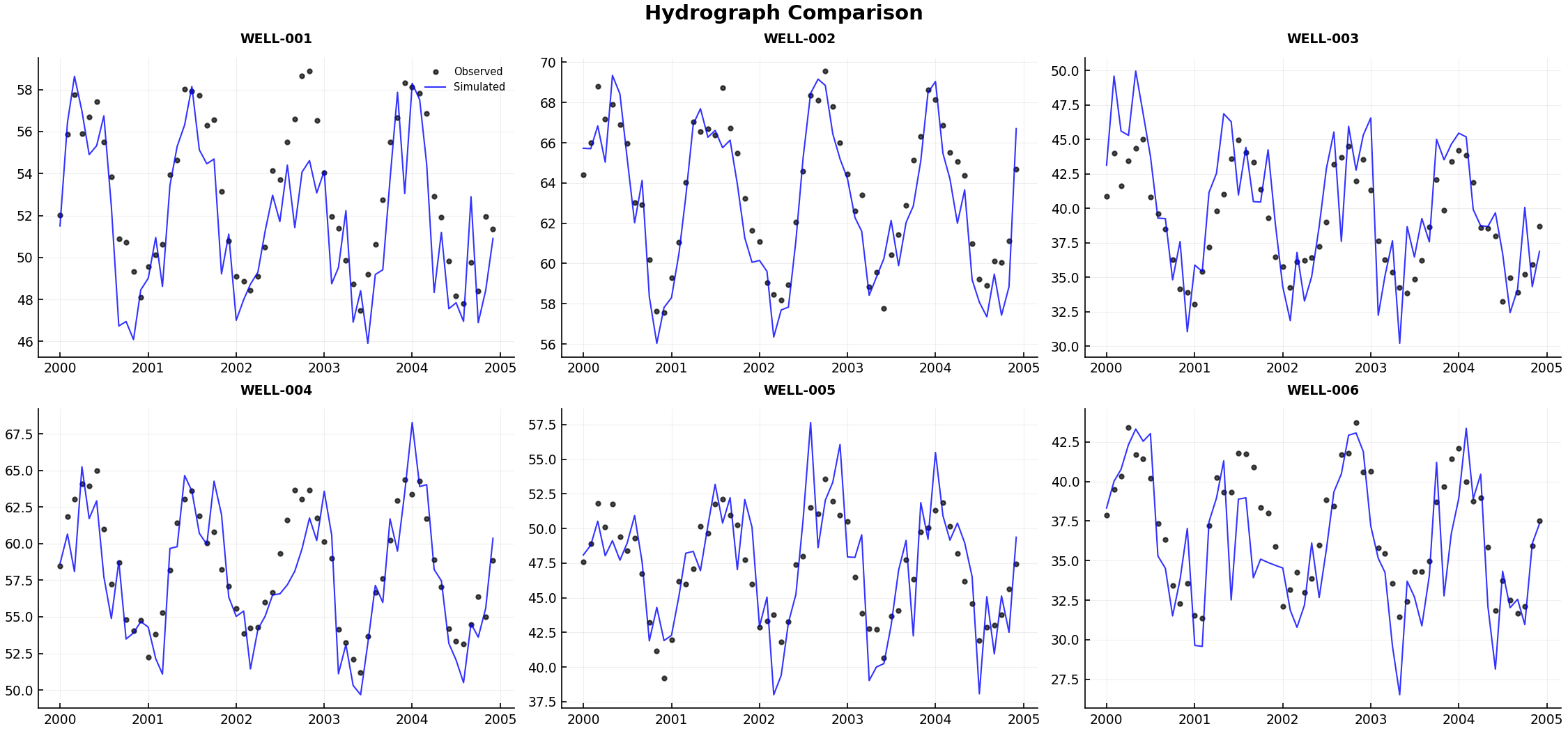
Hydrograph Panel (grid of obs vs sim):
from pyiwfm.visualization.calibration_plots import plot_hydrograph_panel

comparisons = {
    bore_id: (ts.times, obs_ts.values, interp_ts.values)
    for bore_id, (obs_ts, interp_ts) in paired_data.items()
}

fig = plot_hydrograph_panel(
    comparisons,
    n_cols=3,
    max_panels=12,
    output_path=Path("hydrographs.png"),
)
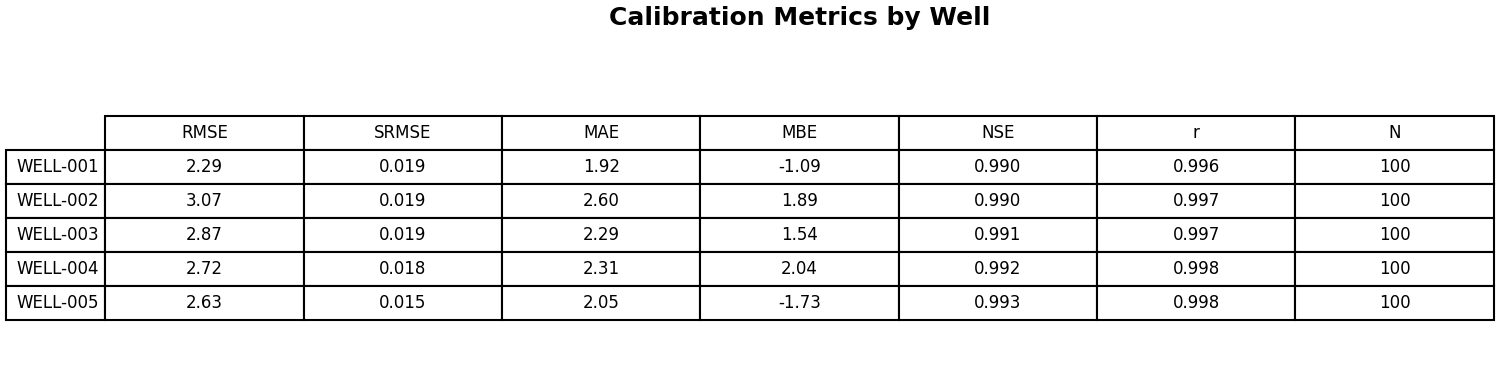
Metrics Table:
from pyiwfm.visualization.calibration_plots import plot_metrics_table

metrics_by_well = {
    bore_id: ComparisonMetrics.compute(obs, sim)
    for bore_id, (obs, sim) in well_comparisons.items()
}

fig = plot_metrics_table(metrics_by_well, output_path=Path("metrics.png"))
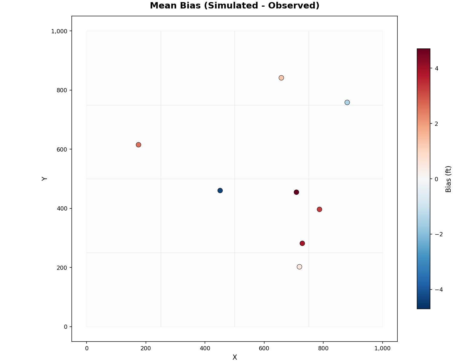
Spatial Bias Map:
from pyiwfm.visualization.plotting import plot_spatial_bias

fig, ax = plot_spatial_bias(
    grid, x_coords, y_coords, bias_values,
    show_mesh=True,
    cmap="RdBu_r",
    title="Mean Bias (Simulated - Observed)",
    units="ft",
)
fig.savefig("spatial_bias.png", dpi=300)
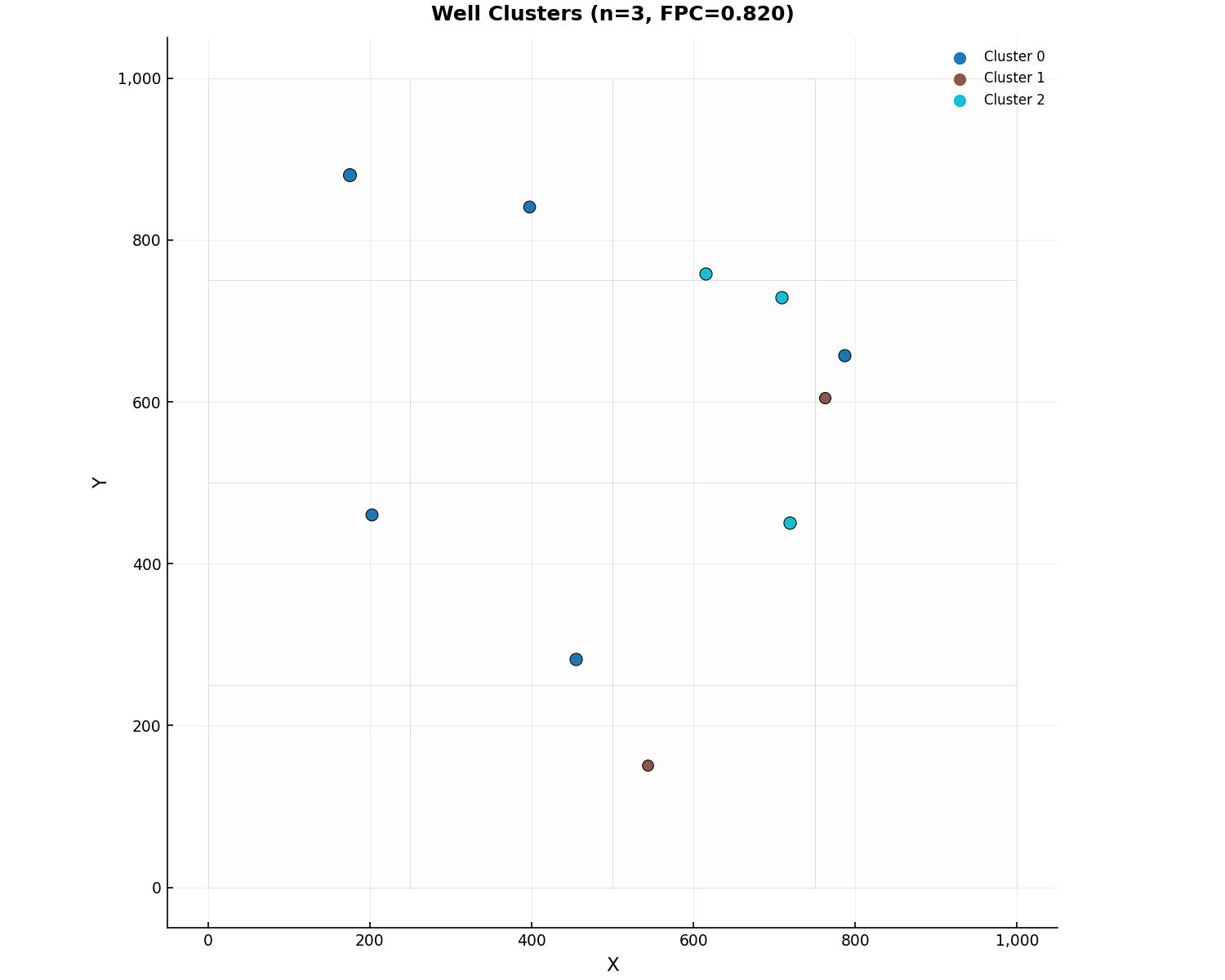
Cluster Map:
from pyiwfm.visualization.calibration_plots import plot_cluster_map

fig, ax = plot_cluster_map(
    well_locations=locations,
    clustering_result=result,
    grid=model.mesh,
)
fig.savefig("cluster_map.png", dpi=300)
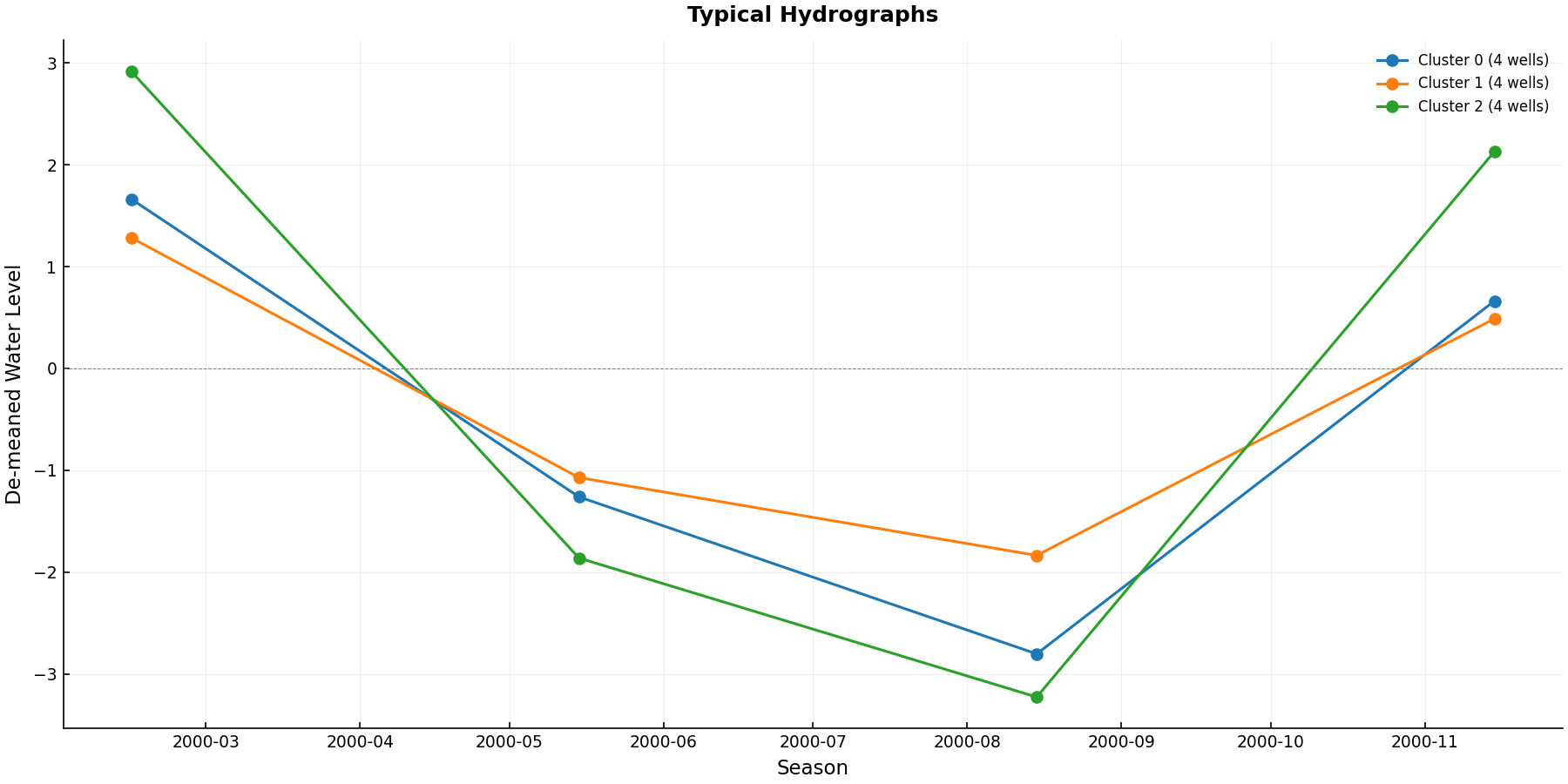
Typical Hydrographs by Cluster:
from pyiwfm.visualization.calibration_plots import plot_typical_hydrographs

fig, ax = plot_typical_hydrographs(typ_result)
fig.savefig("typical_hydrographs.png", dpi=300)
Step 7: Parse SimulationMessages.out#
After running a simulation, parse SimulationMessages.out to extract
warnings, errors, and their spatial locations:
from pyiwfm.io.simulation_messages import SimulationMessagesReader

reader = SimulationMessagesReader("SimulationMessages.out")
result = reader.read()

print(f"Total messages: {len(result.messages)}")
print(f"Warnings: {result.warning_count}")
print(f"Errors: {result.error_count}")

# Filter by severity
from pyiwfm.io.simulation_messages import MessageSeverity

warnings = result.filter_by_severity(MessageSeverity.WARN)
for msg in warnings[:5]:
    print(f"  [{msg.procedure}] {msg.text[:80]}...")
    if msg.node_ids:
        print(f"    Nodes: {msg.node_ids}")

# Get spatial summary (which nodes/elements are most problematic)
spatial = result.get_spatial_summary()
print(f"Nodes with issues: {len(spatial.get('nodes', {}))}")
print(f"Elements with issues: {len(spatial.get('elements', {}))}")
CLI Commands#
pyiwfm provides CLI subcommands for IWFM2OBS and CalcTypHyd:
# Interpolate simulated heads to observation times
pyiwfm iwfm2obs --obs observed.smp --sim simulated.smp --output interp.smp

# Compute typical hydrographs
pyiwfm calctyphyd --water-levels wl.smp --weights weights.txt --output typhyd.smp
Summary#
This tutorial covered:
SMP I/O: Reading and writing IWFM observation files
IWFM2OBS: Time interpolation and multi-layer T-weighted averaging
Model Discovery: Auto-discovering
.outfiles from simulation main fileMulti-layer Wells: Observation well specification, T-weighted averaging,
GW_MultiLayer.outand PEST.insoutputClustering: Fuzzy c-means well clustering with spatial+temporal features
CalcTypHyd: Typical hydrograph computation by cluster
Metrics: Scaled RMSE and standard calibration metrics
Plots: 1:1 plots, residual histograms, hydrograph panels, spatial bias, cluster maps, and publication-quality composite figures
SimulationMessages: Parsing simulation warnings/errors with spatial IDs
Key modules:
pyiwfm.io.smp– SMP file reader/writerpyiwfm.io.hydrograph_reader– IWFM hydrograph.outfile readerpyiwfm.io.simulation_messages– SimulationMessages.out parserpyiwfm.calibration.model_file_discovery– Model file auto-discoverypyiwfm.calibration.obs_well_spec– Observation well specification readerpyiwfm.calibration.iwfm2obs– IWFM2OBS interpolation and model-discovery workflowpyiwfm.calibration.clustering– Fuzzy c-means clusteringpyiwfm.calibration.calctyphyd– Typical hydrograph computationpyiwfm.visualization.plotting– 1:1 and spatial bias plotspyiwfm.visualization.calibration_plots– Composite calibration figures