Visualization Gallery

This gallery showcases pyiwfm’s visualization capabilities using sample models. Each example includes the code used to generate the visualization.

Contents:

• Mesh Visualization
• Scalar Field Visualization
• Stream Network Visualization
• Stratigraphy Visualization
• Time Series Visualization
• Water Budget Visualization
• Mesh Quality Visualization
• Drawdown Maps
• Convergence Visualization

Overview

pyiwfm provides comprehensive visualization tools for:

• Mesh Visualization: Display finite element meshes with nodes, elements, and boundaries

• Scalar Fields: Visualize spatial data like hydraulic head, drawdown, and recharge

• Stream Networks: Display stream node and reach connectivity

• Stratigraphy: Visualize vertical layer structure and aquifer geometry

• Time Series: Plot temporal data from wells, streams, and other monitoring points

• Budget Plots: Display water budget components as bar charts, pie charts, and stacked plots

• Mesh Quality: Visualize element aspect ratios, skewness, and angle distributions

• Drawdown Maps: Diverging colormap drawdown visualization with contours

• Convergence: Iteration count timeseries and mass balance error charts

Quick Start

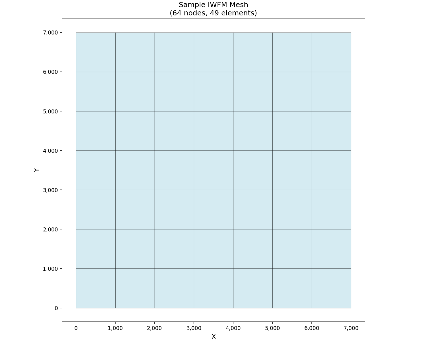
Here’s a quick example showing how to create and visualize a sample mesh:

import matplotlib.pyplot as plt
from pyiwfm.sample_models import create_sample_mesh
from pyiwfm.visualization.plotting import plot_mesh

# Create a sample mesh
mesh = create_sample_mesh(nx=8, ny=8, n_subregions=4)

# Plot mesh
fig, ax = plot_mesh(mesh, show_edges=True, fill_color='lightblue', alpha=0.5)
ax.set_title(f'Sample IWFM Mesh\n({mesh.n_nodes} nodes, {mesh.n_elements} elements)')
plt.show()

(Source code)

All visualizations in pyiwfm are built on matplotlib and return matplotlib objects that can be further customized. See the individual gallery pages for more detailed examples.