Mesh Visualization

This page demonstrates various ways to visualize IWFM finite element meshes using pyiwfm’s visualization tools.

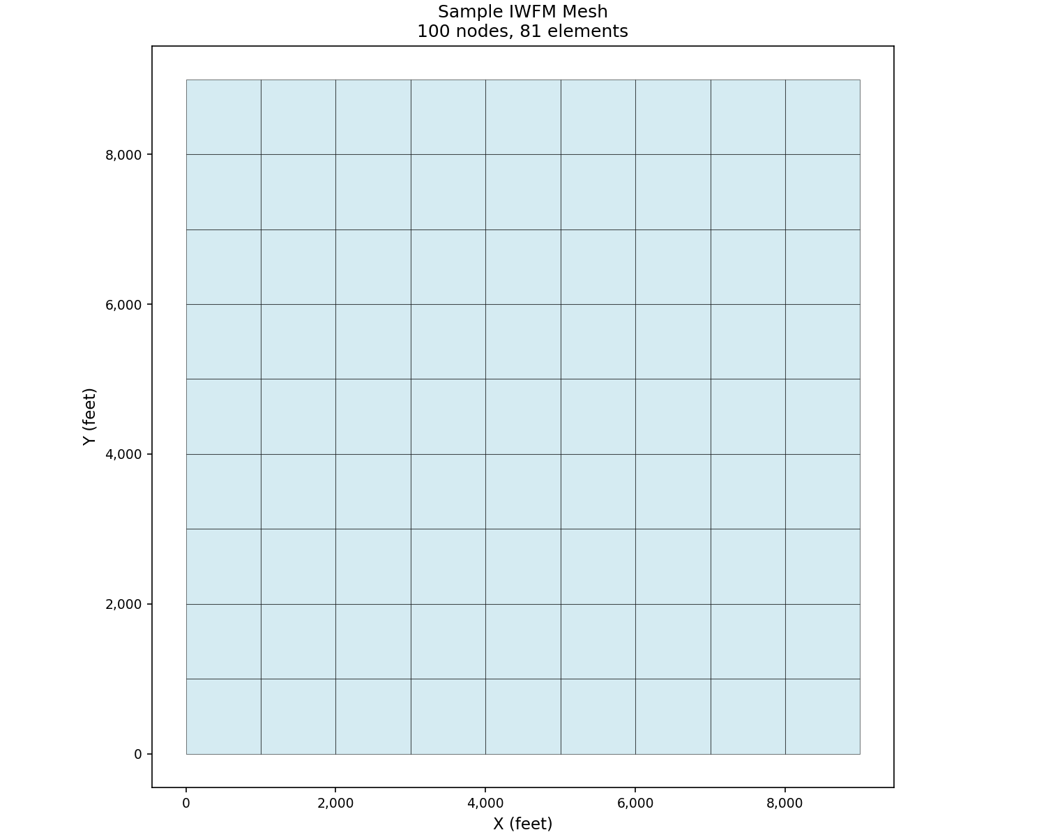
Basic Mesh Display

The simplest way to visualize a mesh is using plot_mesh():

import matplotlib.pyplot as plt
from pyiwfm.sample_models import create_sample_mesh
from pyiwfm.visualization.plotting import plot_mesh

# Create a sample rectangular mesh
mesh = create_sample_mesh(nx=10, ny=10, dx=1000.0, dy=1000.0, n_subregions=4)

fig, ax = plot_mesh(mesh, show_edges=True, edge_color='black',
                    fill_color='lightblue', alpha=0.5)
ax.set_title(f'Sample IWFM Mesh\n{mesh.n_nodes} nodes, {mesh.n_elements} elements')
ax.set_xlabel('X (feet)')
ax.set_ylabel('Y (feet)')
plt.show()

(Source code)

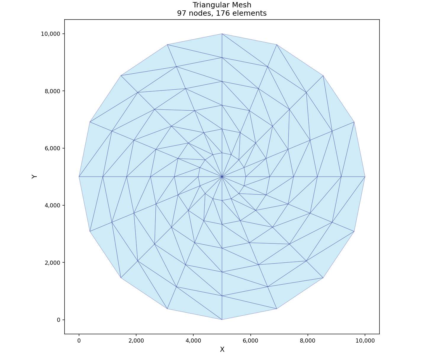
Triangular Mesh

pyiwfm also supports triangular meshes, common in variable-resolution models:

import matplotlib.pyplot as plt
from pyiwfm.sample_models import create_sample_triangular_mesh
from pyiwfm.visualization.plotting import plot_mesh

# Create a radial triangular mesh
mesh = create_sample_triangular_mesh(n_rings=6, n_sectors=16, n_subregions=4)

fig, ax = plot_mesh(mesh, show_edges=True, edge_color='navy', edge_width=0.5,
                    fill_color='skyblue', alpha=0.4)
ax.set_title(f'Triangular Mesh\n{mesh.n_nodes} nodes, {mesh.n_elements} elements')
ax.set_aspect('equal')
plt.show()

(Source code)

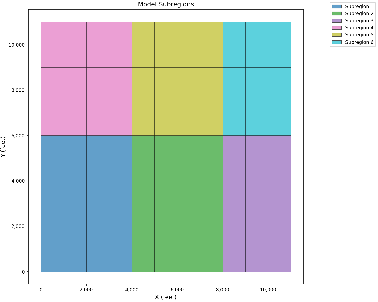
Subregion Visualization

Use plot_elements() with color_by='subregion':

import matplotlib.pyplot as plt
from pyiwfm.sample_models import create_sample_mesh
from pyiwfm.visualization.plotting import plot_elements

mesh = create_sample_mesh(nx=12, ny=12, n_subregions=6)

fig, ax = plot_elements(mesh, color_by='subregion', cmap='tab10',
                         alpha=0.7, edge_color='black', edge_width=0.3)
ax.set_title('Model Subregions')
ax.set_xlabel('X (feet)')
ax.set_ylabel('Y (feet)')
plt.show()

(Source code)

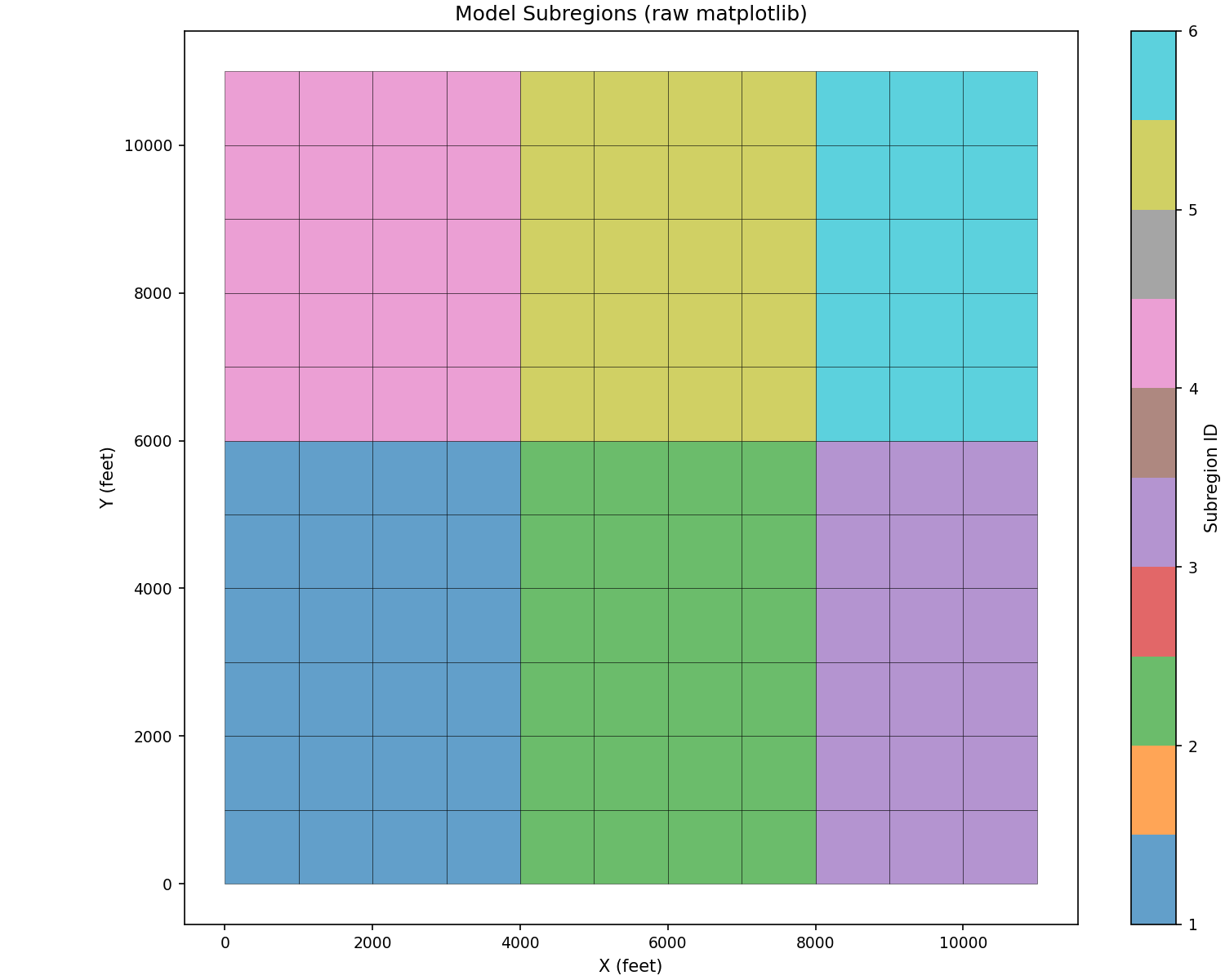
Raw matplotlib alternative for custom coloring:

import matplotlib.pyplot as plt
import numpy as np
from matplotlib.patches import Polygon
from matplotlib.collections import PatchCollection
from pyiwfm.sample_models import create_sample_mesh

mesh = create_sample_mesh(nx=12, ny=12, n_subregions=6)

fig, ax = plt.subplots(figsize=(10, 8))

patches = []
colors = []
for elem in mesh.elements.values():
    verts = [(mesh.nodes[v].x, mesh.nodes[v].y) for v in elem.vertices]
    patches.append(Polygon(verts))
    colors.append(elem.subregion)

p = PatchCollection(patches, alpha=0.7, edgecolor='black', linewidth=0.3)
p.set_array(np.array(colors))
p.set_cmap('tab10')
ax.add_collection(p)
ax.autoscale()
ax.set_aspect('equal')
plt.colorbar(p, ax=ax, label='Subregion ID')
ax.set_title('Model Subregions (raw matplotlib)')
ax.set_xlabel('X (feet)')
ax.set_ylabel('Y (feet)')
plt.show()

(Source code)

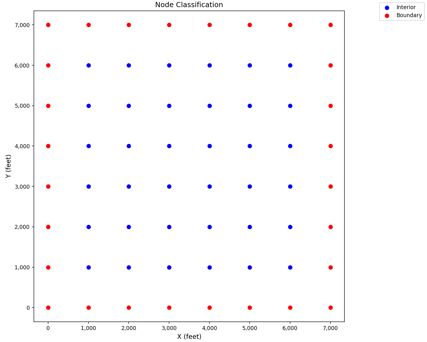
Node Classification

Use plot_nodes() to distinguish boundary and interior nodes:

import matplotlib.pyplot as plt
from pyiwfm.sample_models import create_sample_mesh
from pyiwfm.visualization.plotting import plot_nodes

mesh = create_sample_mesh(nx=8, ny=8, n_subregions=4)

fig, ax = plot_nodes(mesh, highlight_boundary=True,
                      color='blue', boundary_color='red',
                      marker_size=40)
ax.set_title('Node Classification')
ax.set_xlabel('X (feet)')
ax.set_ylabel('Y (feet)')
plt.show()

(Source code)

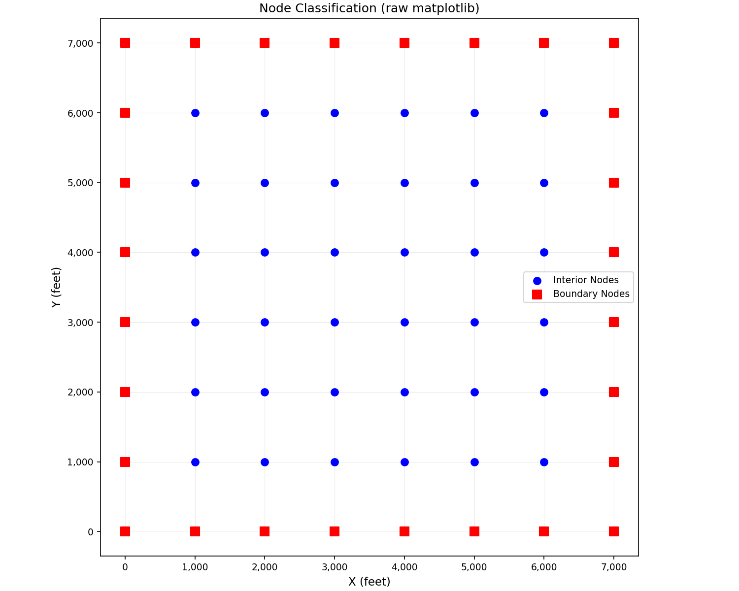
Raw matplotlib alternative with mesh overlay:

import matplotlib.pyplot as plt
from pyiwfm.sample_models import create_sample_mesh
from pyiwfm.visualization.plotting import plot_mesh

mesh = create_sample_mesh(nx=8, ny=8, n_subregions=4)

fig, ax = plot_mesh(mesh, show_edges=True, edge_color='lightgray',
                    fill_color='white', alpha=0.3)

boundary_nodes = [(n.x, n.y) for n in mesh.nodes.values() if n.is_boundary]
interior_nodes = [(n.x, n.y) for n in mesh.nodes.values() if not n.is_boundary]

if interior_nodes:
    ix, iy = zip(*interior_nodes)
    ax.scatter(ix, iy, c='blue', s=50, label='Interior Nodes', zorder=5)
if boundary_nodes:
    bx, by = zip(*boundary_nodes)
    ax.scatter(bx, by, c='red', s=70, marker='s', label='Boundary Nodes', zorder=5)

ax.legend()
ax.set_title('Node Classification (raw matplotlib)')
ax.set_xlabel('X (feet)')
ax.set_ylabel('Y (feet)')
plt.show()

(Source code)

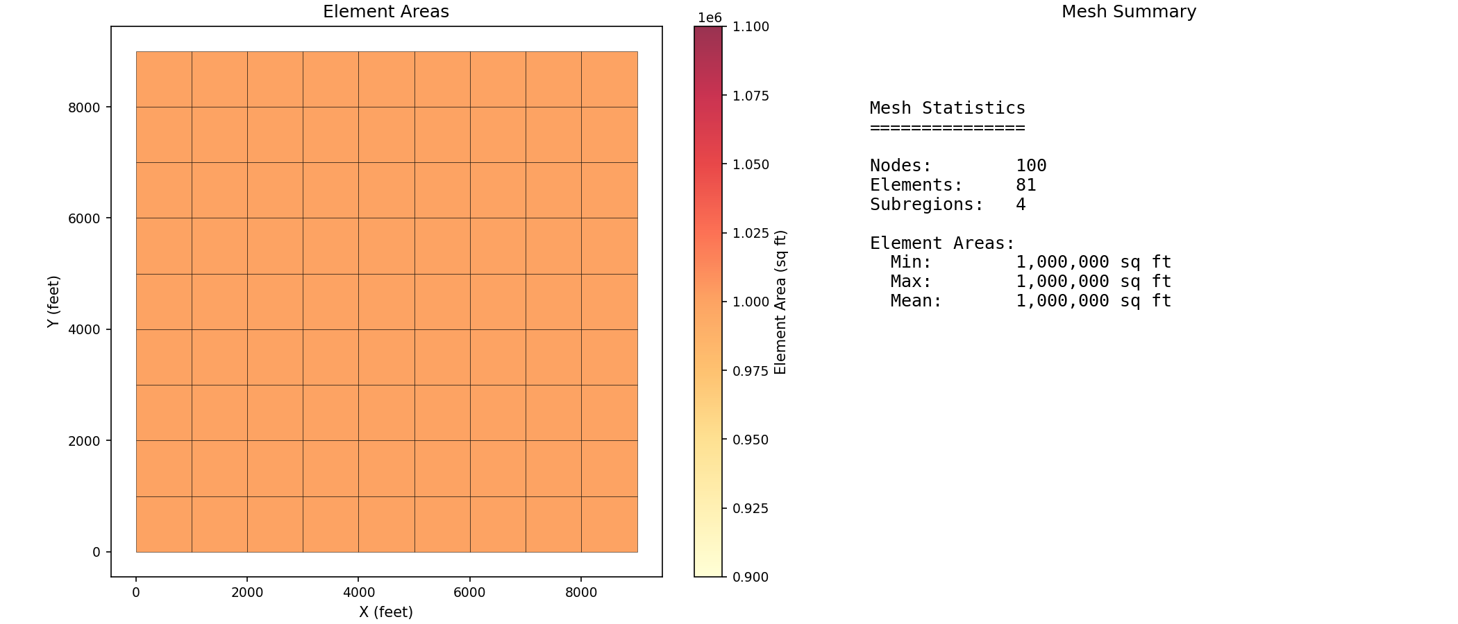
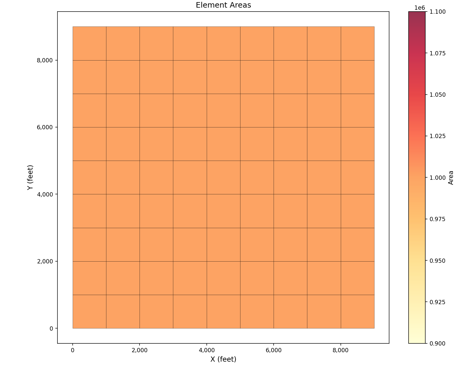
Mesh Statistics

Use plot_elements() with color_by='area' to visualize element sizes:

import matplotlib.pyplot as plt
from pyiwfm.sample_models import create_sample_mesh
from pyiwfm.visualization.plotting import plot_elements

mesh = create_sample_mesh(nx=10, ny=10, n_subregions=4)

fig, ax = plot_elements(mesh, color_by='area', cmap='YlOrRd',
                         alpha=0.8, edge_color='black', edge_width=0.3)
ax.set_title('Element Areas')
ax.set_xlabel('X (feet)')
ax.set_ylabel('Y (feet)')
plt.show()

(Source code)

Two-panel view with statistics summary:

import matplotlib.pyplot as plt
from matplotlib.patches import Polygon
from matplotlib.collections import PatchCollection
import numpy as np
from pyiwfm.sample_models import create_sample_mesh

mesh = create_sample_mesh(nx=10, ny=10, n_subregions=4)

fig, axes = plt.subplots(1, 2, figsize=(14, 6))

elem_areas = []
patches = []
for elem in mesh.elements.values():
    verts = [(mesh.nodes[v].x, mesh.nodes[v].y) for v in elem.vertices]
    patches.append(Polygon(verts))
    elem_areas.append(elem.area)

ax1 = axes[0]
p1 = PatchCollection(patches, alpha=0.8, edgecolor='black', linewidth=0.3)
p1.set_array(np.array(elem_areas))
p1.set_cmap('YlOrRd')
ax1.add_collection(p1)
ax1.autoscale()
ax1.set_aspect('equal')
fig.colorbar(p1, ax=ax1, label='Element Area (sq ft)')
ax1.set_title('Element Areas')
ax1.set_xlabel('X (feet)')
ax1.set_ylabel('Y (feet)')

ax2 = axes[1]
ax2.axis('off')

stats_text = f"""
Mesh Statistics
===============

Nodes:        {mesh.n_nodes:,}
Elements:     {mesh.n_elements:,}
Subregions:   {len(mesh.subregions)}

Element Areas:
  Min:        {min(elem_areas):,.0f} sq ft
  Max:        {max(elem_areas):,.0f} sq ft
  Mean:       {np.mean(elem_areas):,.0f} sq ft
"""
ax2.text(0.1, 0.9, stats_text, transform=ax2.transAxes,
         fontsize=12, verticalalignment='top', family='monospace')
ax2.set_title('Mesh Summary')
plt.show()

(Source code)