Stratigraphy Visualization

This page demonstrates how to visualize the vertical layer structure of IWFM groundwater models.

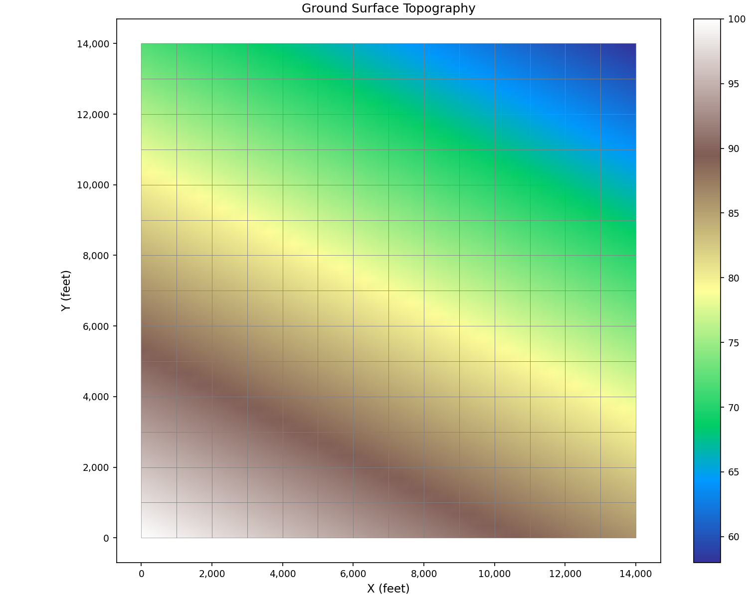
Ground Surface Elevation

Display the ground surface topography:

import matplotlib.pyplot as plt
from pyiwfm.sample_models import create_sample_mesh, create_sample_stratigraphy
from pyiwfm.visualization.plotting import plot_scalar_field

mesh = create_sample_mesh(nx=15, ny=15, n_subregions=4)
strat = create_sample_stratigraphy(mesh, n_layers=3)

fig, ax = plot_scalar_field(mesh, strat.gs_elev, cmap='terrain',
                            figsize=(10, 8))
ax.set_title('Ground Surface Topography')
ax.set_xlabel('X (feet)')
ax.set_ylabel('Y (feet)')
plt.show()

(Source code)

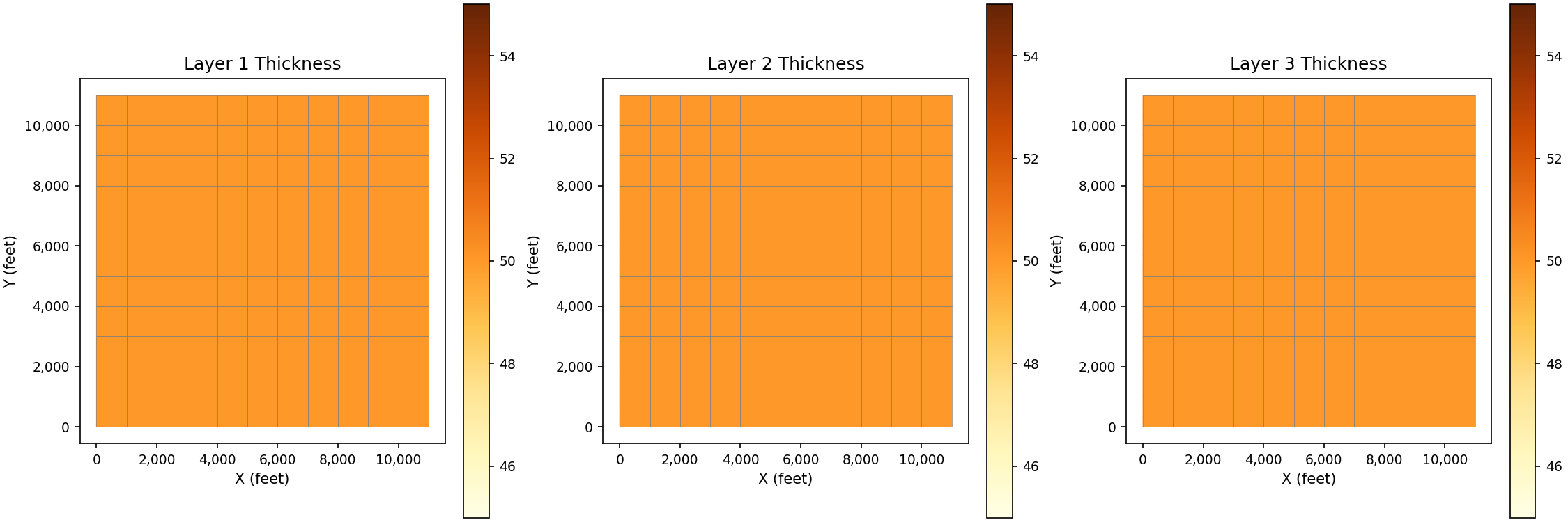
Layer Thickness

Visualize the thickness of each aquifer layer:

import matplotlib.pyplot as plt
from pyiwfm.sample_models import create_sample_mesh, create_sample_stratigraphy
from pyiwfm.visualization.plotting import plot_scalar_field

mesh = create_sample_mesh(nx=12, ny=12, n_subregions=4)
strat = create_sample_stratigraphy(mesh, n_layers=3, layer_thickness=50.0)

fig, axes = plt.subplots(1, 3, figsize=(15, 5))

for i in range(strat.n_layers):
    thickness = strat.get_layer_thickness(i)
    ax = axes[i]
    plot_scalar_field(mesh, thickness, ax=ax, cmap='YlOrBr')
    ax.set_title(f'Layer {i+1} Thickness')
    ax.set_xlabel('X (feet)')
    ax.set_ylabel('Y (feet)')

plt.show()

(Source code)

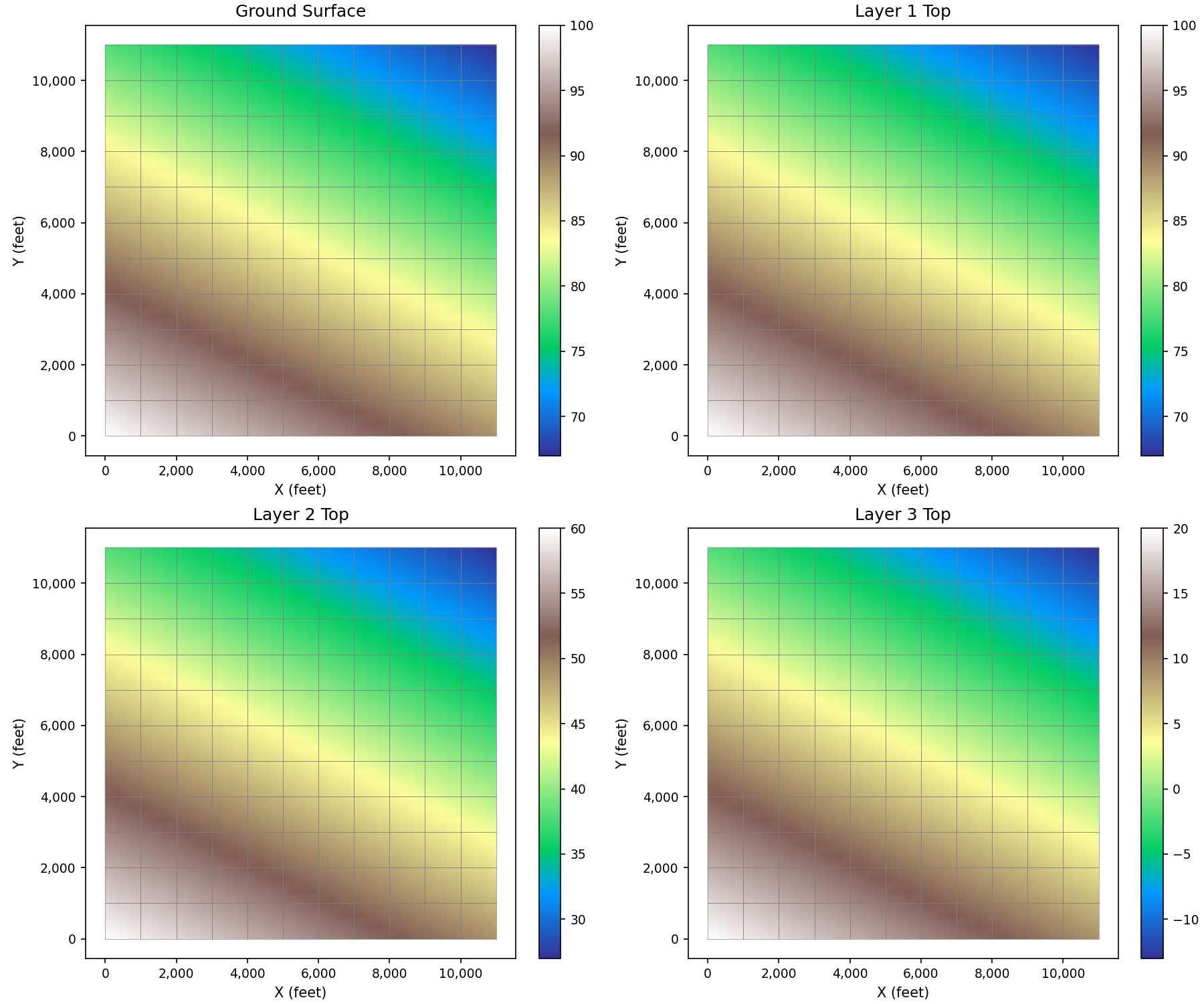
Layer Top Elevations

Show the top elevation of each layer:

import matplotlib.pyplot as plt
from pyiwfm.sample_models import create_sample_mesh, create_sample_stratigraphy
from pyiwfm.visualization.plotting import plot_scalar_field

mesh = create_sample_mesh(nx=12, ny=12, n_subregions=4)
strat = create_sample_stratigraphy(mesh, n_layers=4, layer_thickness=40.0)

fig, axes = plt.subplots(2, 2, figsize=(12, 10))
axes = axes.flatten()

# Ground surface + 3 layer tops
surfaces = [
    ('Ground Surface', strat.gs_elev),
    ('Layer 1 Top', strat.top_elev[:, 0]),
    ('Layer 2 Top', strat.top_elev[:, 1]),
    ('Layer 3 Top', strat.top_elev[:, 2]),
]

for ax, (title, data) in zip(axes, surfaces):
    plot_scalar_field(mesh, data, ax=ax, cmap='terrain')
    ax.set_title(title)
    ax.set_xlabel('X (feet)')
    ax.set_ylabel('Y (feet)')

plt.show()

(Source code)

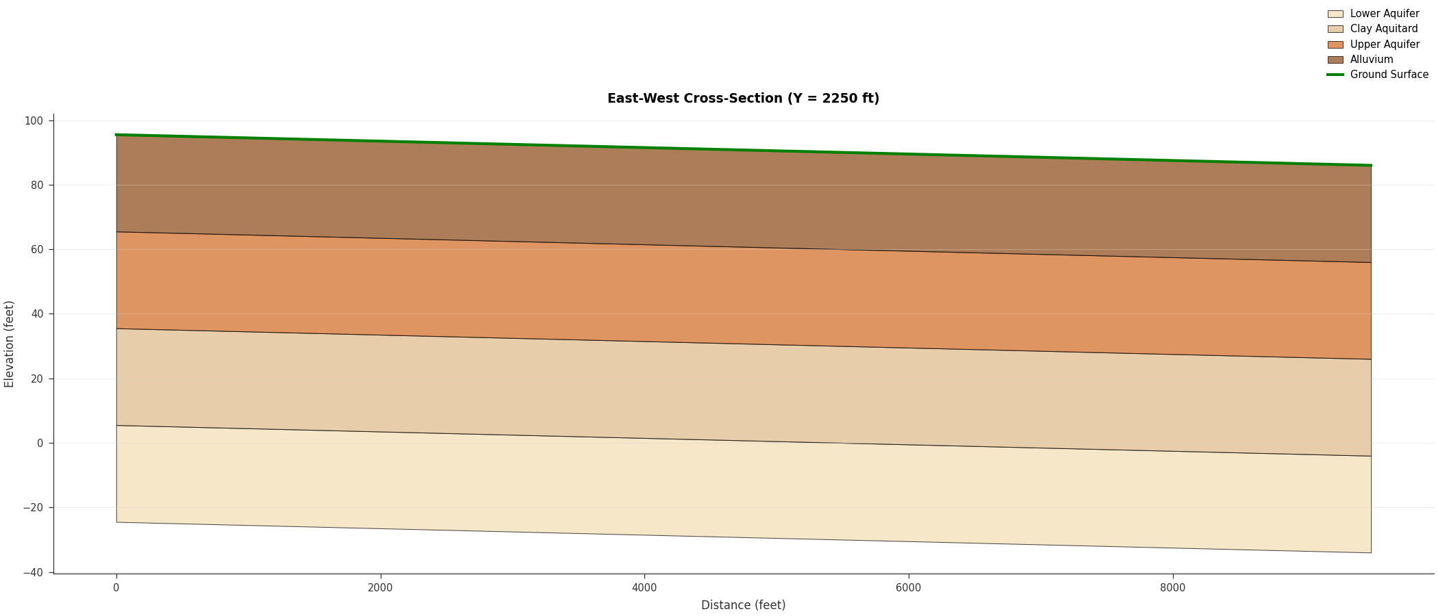
Cross-Section View

Extract a smooth cross-section using finite element interpolation. Unlike node-snapping, this works along any line at any angle:

import matplotlib.pyplot as plt
from pyiwfm.sample_models import create_sample_mesh, create_sample_stratigraphy
from pyiwfm.core.cross_section import CrossSectionExtractor
from pyiwfm.visualization.plotting import plot_cross_section

mesh = create_sample_mesh(nx=20, ny=10, dx=500.0, dy=500.0, n_subregions=4)
strat = create_sample_stratigraphy(mesh, n_layers=4, layer_thickness=30.0)

extractor = CrossSectionExtractor(mesh, strat)
xs = extractor.extract(start=(0, 2250), end=(9500, 2250), n_samples=120)

fig, ax = plot_cross_section(
    xs,
    layer_labels=['Alluvium', 'Upper Aquifer', 'Clay Aquitard', 'Lower Aquifer'],
    title=f'East-West Cross-Section (Y = 2250 ft)',
    figsize=(14, 6),
)
ax.set_xlabel('Distance (feet)')
ax.set_ylabel('Elevation (feet)')
plt.show()

(Source code)

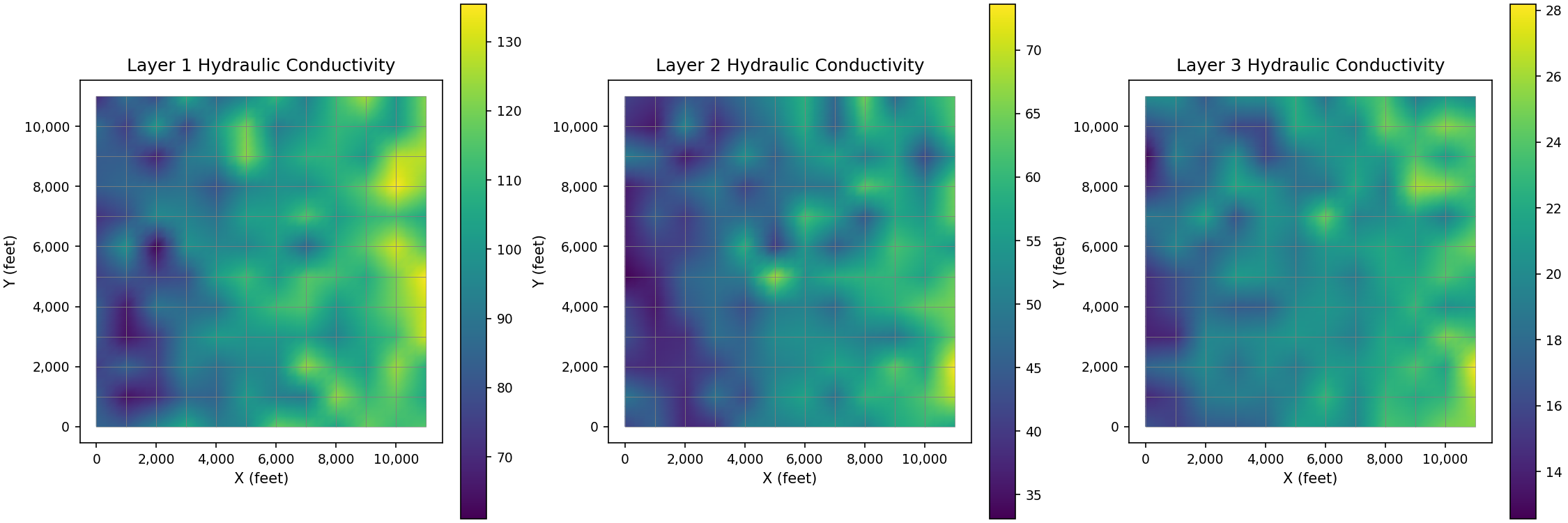
Layer Properties

Display aquifer parameters by layer:

import matplotlib.pyplot as plt
import numpy as np
from pyiwfm.sample_models import create_sample_mesh, create_sample_stratigraphy
from pyiwfm.visualization.plotting import plot_scalar_field

mesh = create_sample_mesh(nx=12, ny=12, n_subregions=4)
strat = create_sample_stratigraphy(mesh, n_layers=3)

# Generate synthetic hydraulic conductivity (varies by layer and position)
n_nodes = mesh.n_nodes
kh = np.zeros((n_nodes, strat.n_layers))

np.random.seed(42)
for layer in range(strat.n_layers):
    base_k = [100.0, 50.0, 20.0][layer]  # Decreasing with depth
    # Add spatial variation
    for i, node in enumerate(mesh.nodes.values()):
        x_norm = node.x / max(n.x for n in mesh.nodes.values())
        kh[i, layer] = base_k * (0.8 + 0.4 * x_norm) + np.random.normal(0, base_k * 0.1)

fig, axes = plt.subplots(1, 3, figsize=(15, 5))

for i in range(strat.n_layers):
    ax = axes[i]
    plot_scalar_field(mesh, kh[:, i], ax=ax, cmap='viridis')
    ax.set_title(f'Layer {i+1} Hydraulic Conductivity')
    ax.set_xlabel('X (feet)')
    ax.set_ylabel('Y (feet)')

plt.show()

(Source code)

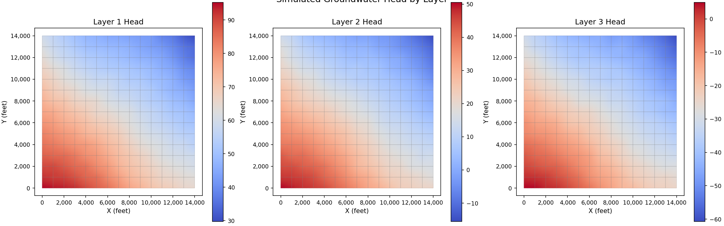
Head Distribution by Layer

Visualize simulated groundwater head across each aquifer layer:

import matplotlib.pyplot as plt
import numpy as np
from pyiwfm.sample_models import create_sample_mesh, create_sample_stratigraphy
from pyiwfm.visualization.plotting import plot_scalar_field

mesh = create_sample_mesh(nx=15, ny=15, n_subregions=4)
strat = create_sample_stratigraphy(mesh, n_layers=3, layer_thickness=40.0)
n_nodes = mesh.n_nodes

# Generate synthetic head values for each layer
# Head generally declines from recharge area (east) to discharge (west)
np.random.seed(42)
x_coords = np.array([n.x for n in mesh.nodes.values()])
y_coords = np.array([n.y for n in mesh.nodes.values()])
x_norm = (x_coords - x_coords.min()) / (x_coords.max() - x_coords.min())
y_norm = (y_coords - y_coords.min()) / (y_coords.max() - y_coords.min())

head = np.zeros((n_nodes, strat.n_layers))
for layer in range(strat.n_layers):
    base = strat.top_elev[:, layer] - 5.0 * (layer + 1)
    gradient = -15.0 * x_norm - 8.0 * y_norm
    mounding = 3.0 * np.sin(2 * np.pi * x_norm) * np.cos(np.pi * y_norm)
    head[:, layer] = base + gradient + mounding + np.random.normal(0, 0.5, n_nodes)

fig, axes = plt.subplots(1, 3, figsize=(16, 5))

for i in range(strat.n_layers):
    ax = axes[i]
    plot_scalar_field(mesh, head[:, i], ax=ax, cmap='coolwarm',
                      edge_color='gray', edge_width=0.15)
    ax.set_title(f'Layer {i+1} Head')
    ax.set_xlabel('X (feet)')
    ax.set_ylabel('Y (feet)')

plt.suptitle('Simulated Groundwater Head by Layer', fontsize=14, y=1.02)
plt.show()

(Source code)

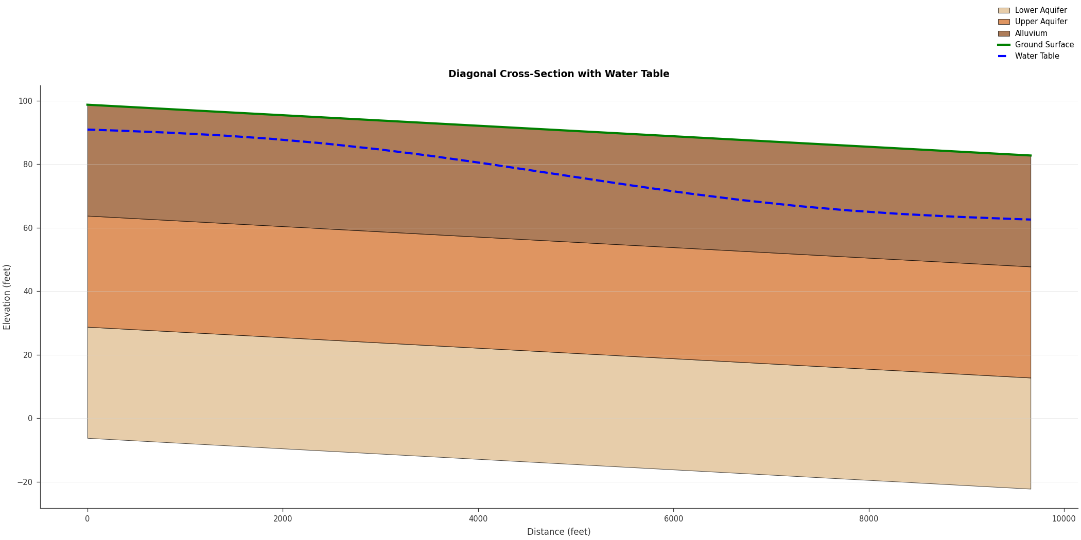
Head and Stratigraphy Cross-Section

Overlay the water table on a stratigraphic cross-section using FE-interpolated extraction along a diagonal line:

import matplotlib.pyplot as plt
import numpy as np
from pyiwfm.sample_models import create_sample_mesh, create_sample_stratigraphy
from pyiwfm.core.cross_section import CrossSectionExtractor
from pyiwfm.visualization.plotting import plot_cross_section

mesh = create_sample_mesh(nx=20, ny=10, dx=500.0, dy=500.0, n_subregions=4)
strat = create_sample_stratigraphy(mesh, n_layers=3, layer_thickness=35.0)

# Extract a diagonal cross-section
extractor = CrossSectionExtractor(mesh, strat)
xs = extractor.extract(start=(250, 500), end=(9250, 4000), n_samples=150)

# Generate synthetic water table and interpolate onto cross-section
n_nodes = mesh.n_nodes
x_coords = np.array([n.x for n in mesh.nodes.values()])
x_norm = (x_coords - x_coords.min()) / (x_coords.max() - x_coords.min())
wt = strat.gs_elev - 8.0 - 12.0 * x_norm + 3.0 * np.sin(2 * np.pi * x_norm)
extractor.interpolate_scalar(xs, wt, 'Water Table')

fig, ax = plot_cross_section(
    xs,
    layer_colors=['#8B4513', '#D2691E', '#DEB887'],
    layer_labels=['Alluvium', 'Upper Aquifer', 'Lower Aquifer'],
    scalar_name='Water Table',
    title='Diagonal Cross-Section with Water Table',
    figsize=(14, 7),
)
ax.set_xlabel('Distance (feet)')
ax.set_ylabel('Elevation (feet)')
plt.show()

(Source code)

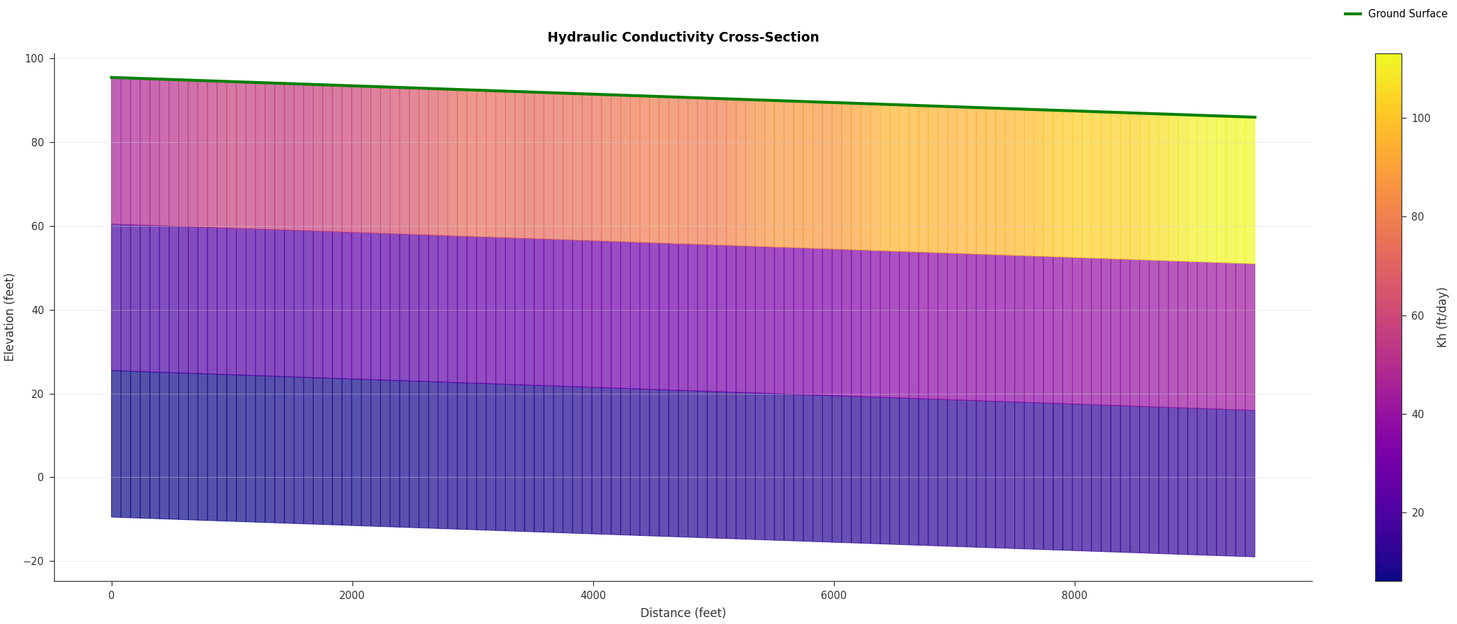
Hydraulic Conductivity Cross-Section

Color-map each layer band by interpolated hydraulic conductivity:

import matplotlib.pyplot as plt
import numpy as np
from pyiwfm.sample_models import create_sample_mesh, create_sample_stratigraphy
from pyiwfm.core.cross_section import CrossSectionExtractor
from pyiwfm.visualization.plotting import plot_cross_section

mesh = create_sample_mesh(nx=20, ny=10, dx=500.0, dy=500.0, n_subregions=4)
strat = create_sample_stratigraphy(mesh, n_layers=3, layer_thickness=35.0)
n_nodes = mesh.n_nodes

# Build synthetic Kh field (n_nodes, n_layers)
np.random.seed(42)
kh = np.zeros((n_nodes, strat.n_layers))
for layer in range(strat.n_layers):
    base_k = [80.0, 30.0, 10.0][layer]
    for i, node in enumerate(mesh.nodes.values()):
        x_norm = node.x / max(n.x for n in mesh.nodes.values())
        kh[i, layer] = base_k * (0.6 + 0.8 * x_norm) + np.random.normal(0, base_k * 0.05)

extractor = CrossSectionExtractor(mesh, strat)
xs = extractor.extract(start=(0, 2250), end=(9500, 2250), n_samples=120)
extractor.interpolate_layer_property(xs, kh, 'Kh (ft/day)')

fig, ax = plot_cross_section(
    xs,
    layer_property_name='Kh (ft/day)',
    layer_property_cmap='plasma',
    title='Hydraulic Conductivity Cross-Section',
    figsize=(14, 6),
)
ax.set_xlabel('Distance (feet)')
ax.set_ylabel('Elevation (feet)')
plt.show()

(Source code)

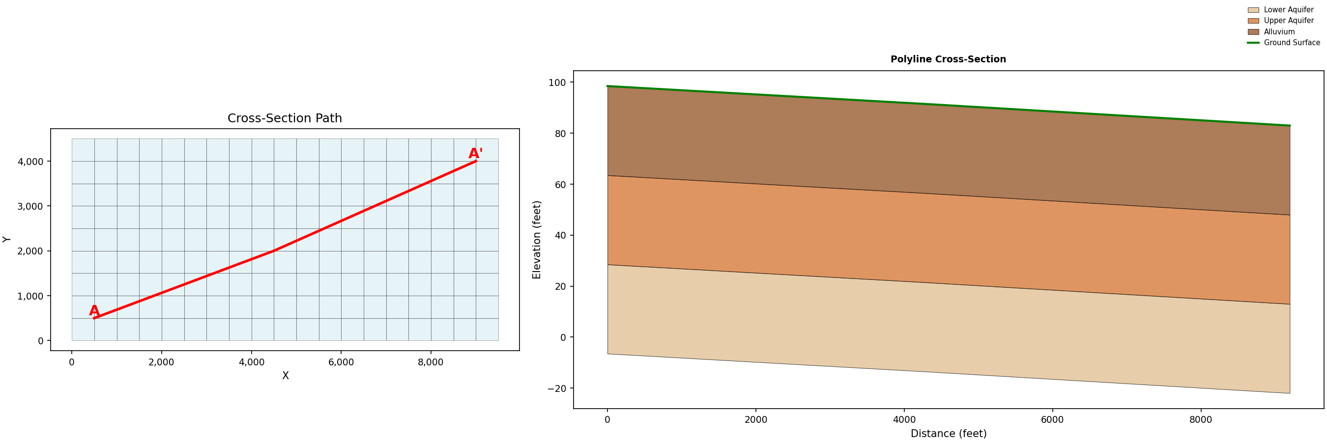
Polyline Cross-Section

Extract along a multi-segment path through the model domain:

import matplotlib.pyplot as plt
from pyiwfm.sample_models import create_sample_mesh, create_sample_stratigraphy
from pyiwfm.core.cross_section import CrossSectionExtractor
from pyiwfm.visualization.plotting import plot_cross_section, plot_cross_section_location

mesh = create_sample_mesh(nx=20, ny=10, dx=500.0, dy=500.0, n_subregions=4)
strat = create_sample_stratigraphy(mesh, n_layers=3, layer_thickness=35.0)

waypoints = [(500, 500), (4500, 2000), (9000, 4000)]
extractor = CrossSectionExtractor(mesh, strat)
xs = extractor.extract_polyline(waypoints, n_samples_per_segment=60)

fig, (ax1, ax2) = plt.subplots(1, 2, figsize=(18, 6),
                                gridspec_kw={'width_ratios': [1, 1.6]})

# Plan view showing the polyline path on the mesh
plot_cross_section_location(mesh, xs, ax=ax1)
ax1.set_title('Cross-Section Path')

# Profile view
plot_cross_section(
    xs, ax=ax2,
    layer_labels=['Alluvium', 'Upper Aquifer', 'Lower Aquifer'],
    title='Polyline Cross-Section',
)
ax2.set_xlabel('Distance (feet)')
ax2.set_ylabel('Elevation (feet)')

plt.show()

(Source code)

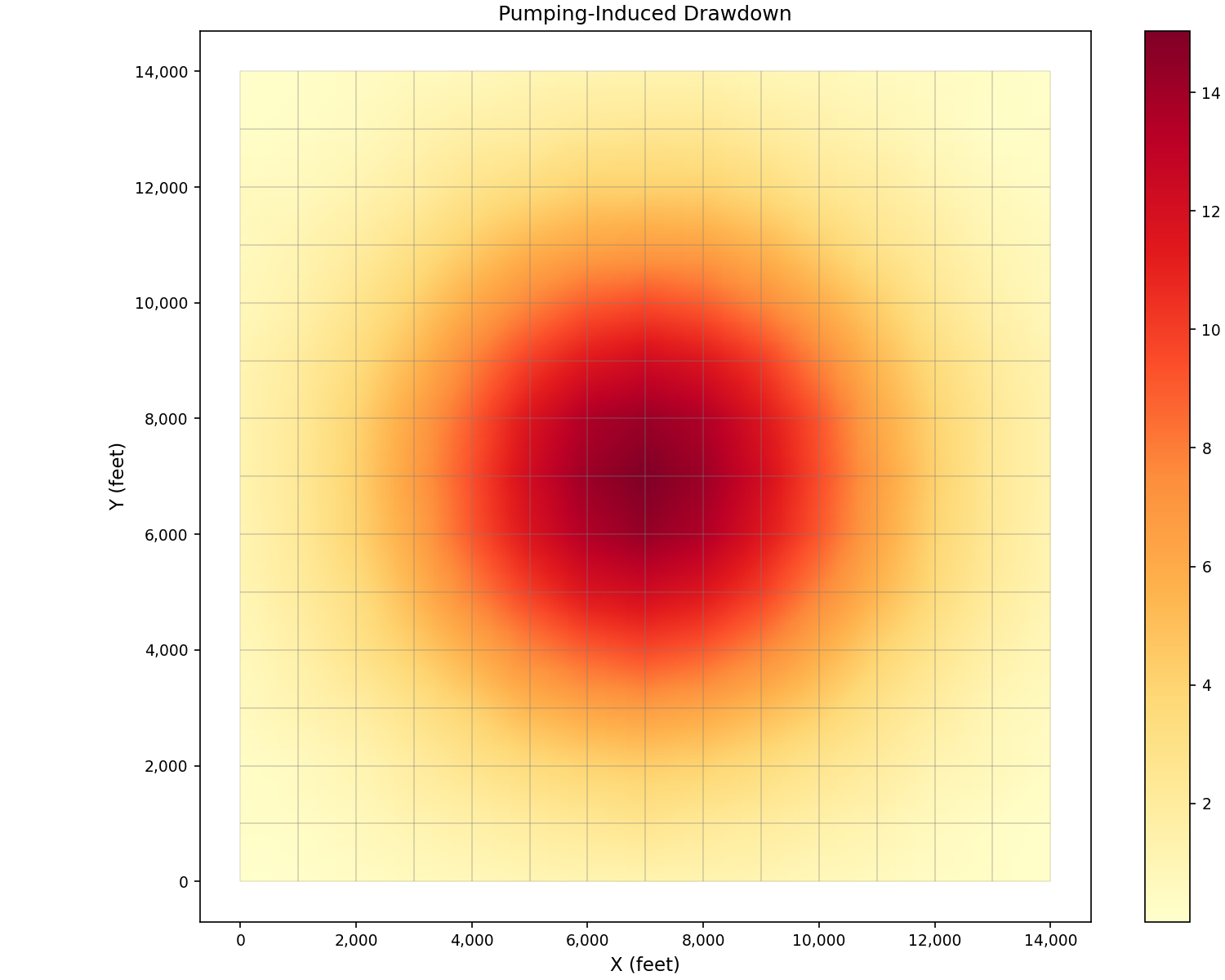
Drawdown from Pumping

Visualize pumping-induced drawdown as a scalar field on the mesh:

import matplotlib.pyplot as plt
from pyiwfm.sample_models import create_sample_mesh, create_sample_scalar_field
from pyiwfm.visualization.plotting import plot_scalar_field

mesh = create_sample_mesh(nx=15, ny=15, n_subregions=4)

# Generate drawdown field (cone of depression centred in domain)
drawdown = create_sample_scalar_field(mesh, field_type='drawdown', noise_level=0.02)

fig, ax = plot_scalar_field(mesh, drawdown, cmap='YlOrRd',
                            edge_color='gray', edge_width=0.15,
                            figsize=(10, 8))
ax.set_title('Pumping-Induced Drawdown')
ax.set_xlabel('X (feet)')
ax.set_ylabel('Y (feet)')
plt.show()

(Source code)

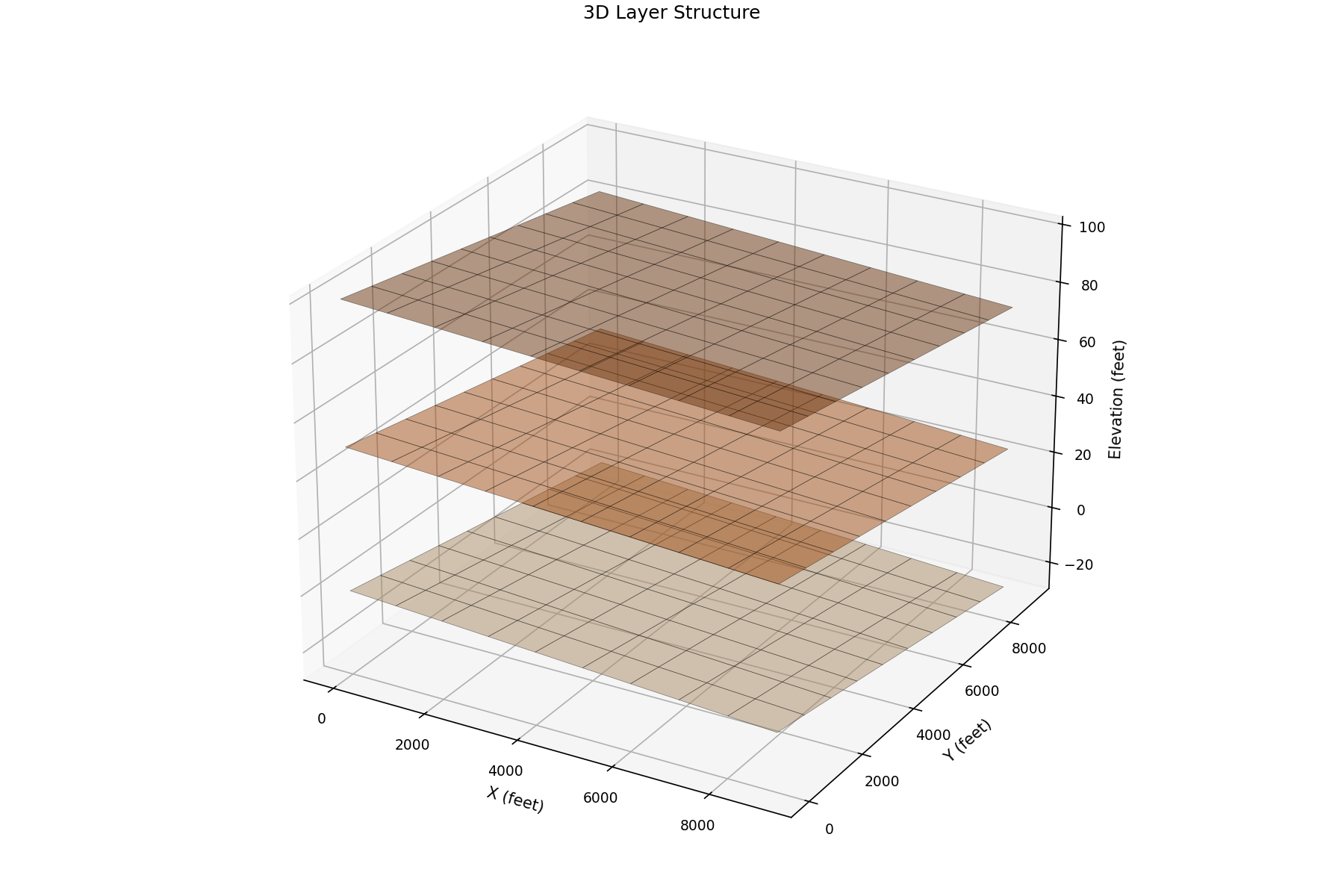
3D Fence Diagram Concept

Display conceptual 3D structure using multiple cross-sections:

import matplotlib.pyplot as plt
import numpy as np
from mpl_toolkits.mplot3d import Axes3D
from pyiwfm.sample_models import create_sample_mesh, create_sample_stratigraphy

mesh = create_sample_mesh(nx=10, ny=10, dx=1000.0, dy=1000.0, n_subregions=4)
strat = create_sample_stratigraphy(mesh, n_layers=3, layer_thickness=50.0)

fig = plt.figure(figsize=(12, 8))
ax = fig.add_subplot(111, projection='3d')

colors = ['#8B4513', '#D2691E', '#DEB887']

# Plot layer surfaces
x_unique = sorted(set(n.x for n in mesh.nodes.values()))
y_unique = sorted(set(n.y for n in mesh.nodes.values()))
X, Y = np.meshgrid(x_unique, y_unique)

for layer in range(strat.n_layers):
    Z_top = np.zeros_like(X)
    Z_bot = np.zeros_like(X)

    for i, xi in enumerate(x_unique):
        for j, yi in enumerate(y_unique):
            # Find nearest node
            min_dist = float('inf')
            nearest_idx = 0
            for idx, node in enumerate(mesh.nodes.values()):
                dist = (node.x - xi)**2 + (node.y - yi)**2
                if dist < min_dist:
                    min_dist = dist
                    nearest_idx = idx

            Z_top[j, i] = strat.top_elev[nearest_idx, layer]
            Z_bot[j, i] = strat.bottom_elev[nearest_idx, layer]

    # Plot top surface
    ax.plot_surface(X, Y, Z_top, alpha=0.5, color=colors[layer % len(colors)],
                    edgecolor='black', linewidth=0.3)

ax.set_xlabel('X (feet)')
ax.set_ylabel('Y (feet)')
ax.set_zlabel('Elevation (feet)')
ax.set_title('3D Layer Structure')

# Set viewing angle
ax.view_init(elev=25, azim=-60)

plt.show()

(Source code)