Convergence Visualization#
Visualize model convergence behavior and mass balance errors using synthetic
data that mimics IWFM SimulationMessages.out patterns.
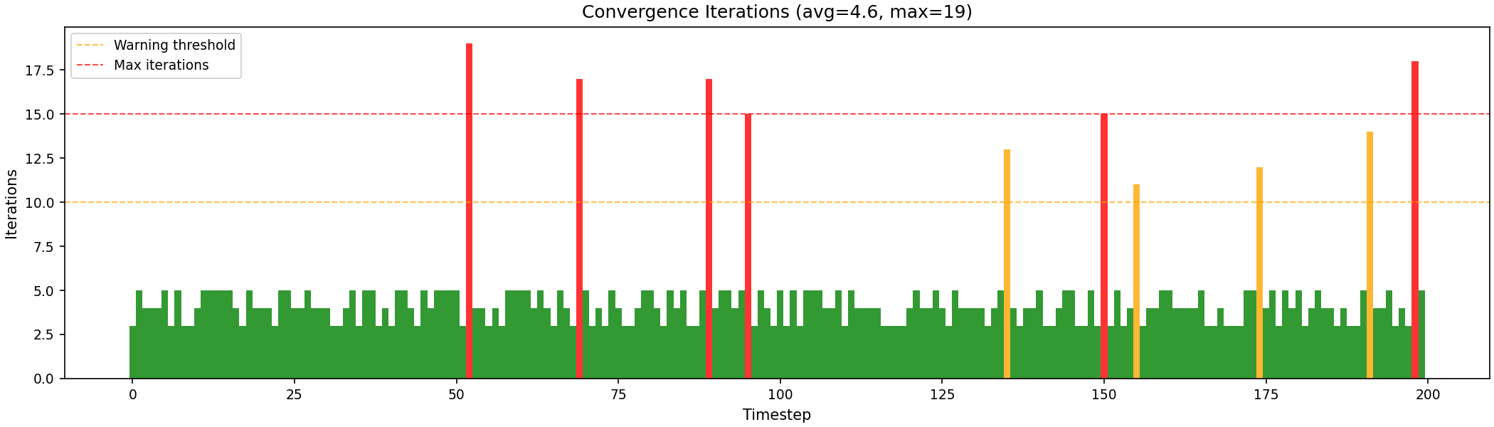
Iteration Count Timeseries#
Plot the number of solver iterations per timestep:
import matplotlib.pyplot as plt
import numpy as np

rng = np.random.default_rng(42)
n_timesteps = 200

# Synthetic iteration counts — mostly 3-5, occasional spikes
base_iters = rng.integers(3, 6, size=n_timesteps)
spikes = rng.choice(n_timesteps, size=10, replace=False)
base_iters[spikes] = rng.integers(10, 20, size=10)

fig, ax = plt.subplots(figsize=(14, 4))
colors = ['green' if i < 10 else 'orange' if i < 15 else 'red' for i in base_iters]
ax.bar(range(n_timesteps), base_iters, color=colors, width=1.0, alpha=0.8)
ax.axhline(10, color='orange', linestyle='--', linewidth=1, alpha=0.7, label='Warning threshold')
ax.axhline(15, color='red', linestyle='--', linewidth=1, alpha=0.7, label='Max iterations')
ax.set_xlabel('Timestep')
ax.set_ylabel('Iterations')
ax.set_title(f'Convergence Iterations (avg={base_iters.mean():.1f}, max={base_iters.max()})')
ax.legend()
plt.show()
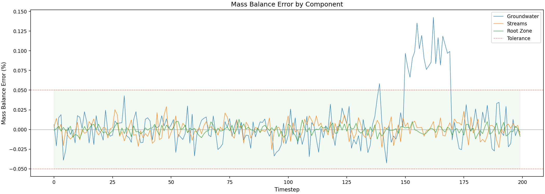
Mass Balance Error Over Time#
Track mass balance discrepancy across multiple model components:
import matplotlib.pyplot as plt
import numpy as np

rng = np.random.default_rng(42)
n_timesteps = 200
timesteps = np.arange(n_timesteps)

# Synthetic mass balance errors for three components
gw_error = rng.normal(0, 0.02, n_timesteps)
gw_error[150:170] += 0.1  # period of higher error
stream_error = rng.normal(0, 0.01, n_timesteps)
rz_error = rng.normal(0, 0.005, n_timesteps)

fig, ax = plt.subplots(figsize=(14, 5))
ax.plot(timesteps, gw_error, label='Groundwater', linewidth=0.8, alpha=0.9)
ax.plot(timesteps, stream_error, label='Streams', linewidth=0.8, alpha=0.9)
ax.plot(timesteps, rz_error, label='Root Zone', linewidth=0.8, alpha=0.9)
ax.axhline(0, color='gray', linestyle='-', linewidth=0.5)
ax.axhline(0.05, color='red', linestyle='--', linewidth=0.8, alpha=0.5, label='Tolerance')
ax.axhline(-0.05, color='red', linestyle='--', linewidth=0.8, alpha=0.5)
ax.fill_between(timesteps, -0.05, 0.05, alpha=0.05, color='green')
ax.set_xlabel('Timestep')
ax.set_ylabel('Mass Balance Error (%)')
ax.set_title('Mass Balance Error by Component')
ax.legend()
plt.show()
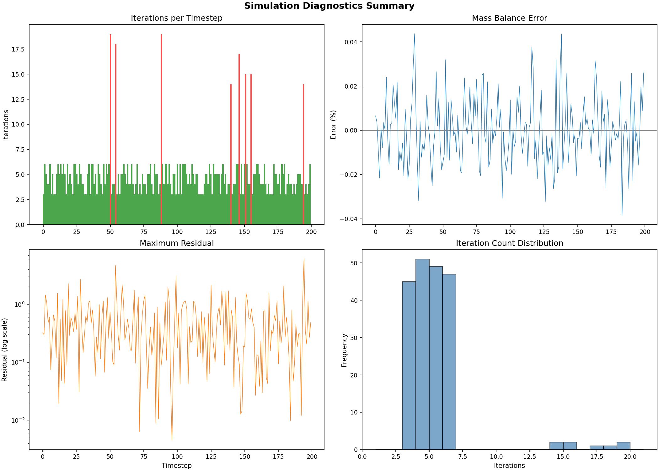
Combined Diagnostics Dashboard#
A multi-panel summary of simulation health:
import matplotlib.pyplot as plt
import numpy as np

rng = np.random.default_rng(42)
n = 200

iters = rng.integers(3, 7, size=n)
iters[rng.choice(n, 8, replace=False)] = rng.integers(12, 20, size=8)

mb_error = rng.normal(0, 0.015, n)
residuals = rng.exponential(0.5, n)
residuals[iters > 10] *= 3

fig, axes = plt.subplots(2, 2, figsize=(14, 10))

# Iterations
ax = axes[0, 0]
ax.bar(range(n), iters, width=1.0, alpha=0.7,
       color=['green' if i < 10 else 'red' for i in iters])
ax.set_title('Iterations per Timestep')
ax.set_ylabel('Iterations')

# Mass balance
ax = axes[0, 1]
ax.plot(mb_error, linewidth=0.7, color='tab:blue')
ax.axhline(0, color='gray', linestyle='-', linewidth=0.5)
ax.set_title('Mass Balance Error')
ax.set_ylabel('Error (%)')

# Max residual
ax = axes[1, 0]
ax.semilogy(residuals, linewidth=0.7, color='tab:orange')
ax.set_title('Maximum Residual')
ax.set_xlabel('Timestep')
ax.set_ylabel('Residual (log scale)')

# Iteration histogram
ax = axes[1, 1]
ax.hist(iters, bins=range(1, 22), edgecolor='black', alpha=0.7, color='steelblue')
ax.set_title('Iteration Count Distribution')
ax.set_xlabel('Iterations')
ax.set_ylabel('Frequency')

plt.suptitle('Simulation Diagnostics Summary', fontsize=14, fontweight='bold')
plt.show()