Stream Network Visualization#
This page demonstrates how to visualize stream networks and stream-aquifer interactions in IWFM models.
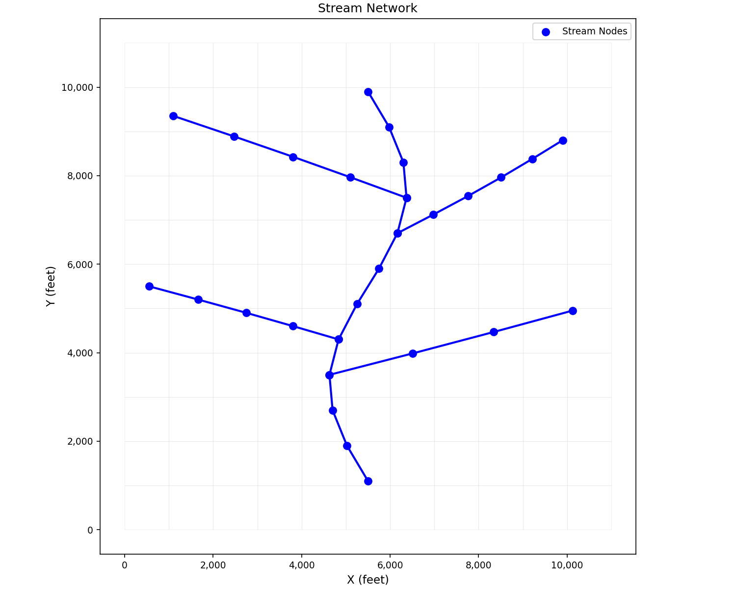
Basic Stream Network#
Display stream nodes and reaches over the model mesh. When working with a
full model that has an AppStream object, use
plot_streams():
from pyiwfm.visualization.plotting import plot_mesh, plot_streams

fig, ax = plot_mesh(grid, show_edges=True, edge_color='lightgray', alpha=0.3)
plot_streams(model.streams, ax=ax, show_nodes=True)
plt.show()
With sample synthetic data, the raw matplotlib approach works directly:
import matplotlib.pyplot as plt
from pyiwfm.sample_models import create_sample_mesh, create_sample_stream_network
from pyiwfm.visualization.plotting import plot_mesh

mesh = create_sample_mesh(nx=12, ny=12, n_subregions=4)
stream_nodes, reaches = create_sample_stream_network(mesh)

fig, ax = plot_mesh(mesh, show_edges=True, edge_color='lightgray',
                    fill_color='white', alpha=0.3)

for from_idx, to_idx in reaches:
    x1, y1 = stream_nodes[from_idx]
    x2, y2 = stream_nodes[to_idx]
    ax.plot([x1, x2], [y1, y2], 'b-', linewidth=2, zorder=3)

sx, sy = zip(*stream_nodes)
ax.scatter(sx, sy, c='blue', s=50, zorder=4, label='Stream Nodes')

ax.legend()
ax.set_title('Stream Network')
ax.set_xlabel('X (feet)')
ax.set_ylabel('Y (feet)')
plt.show()
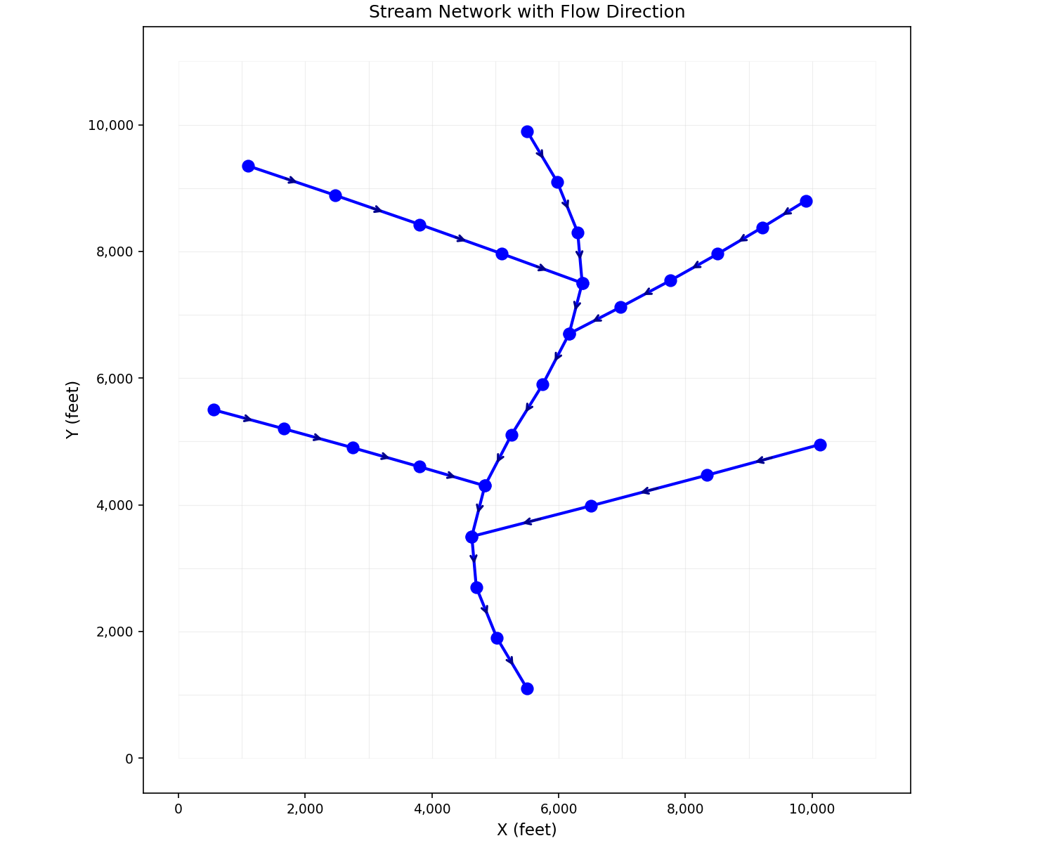
Stream Network with Flow Direction#
Show flow direction using arrows:
import matplotlib.pyplot as plt
from pyiwfm.sample_models import create_sample_mesh, create_sample_stream_network
from pyiwfm.visualization.plotting import plot_mesh

mesh = create_sample_mesh(nx=12, ny=12, n_subregions=4)
stream_nodes, reaches = create_sample_stream_network(mesh)

fig, ax = plot_mesh(mesh, show_edges=True, edge_color='lightgray',
                    fill_color='white', alpha=0.2)

for from_idx, to_idx in reaches:
    x1, y1 = stream_nodes[from_idx]
    x2, y2 = stream_nodes[to_idx]

    ax.plot([x1, x2], [y1, y2], 'b-', linewidth=2, zorder=3)

    mx, my = (x1 + x2) / 2, (y1 + y2) / 2
    dx, dy = x2 - x1, y2 - y1
    ax.annotate('', xy=(mx + dx*0.1, my + dy*0.1),
                xytext=(mx - dx*0.1, my - dy*0.1),
                arrowprops=dict(arrowstyle='->', color='darkblue', lw=1.5),
                zorder=5)

for i, (x, y) in enumerate(stream_nodes):
    ax.scatter(x, y, c='blue', s=60, zorder=4)

ax.set_title('Stream Network with Flow Direction')
ax.set_xlabel('X (feet)')
ax.set_ylabel('Y (feet)')
plt.show()
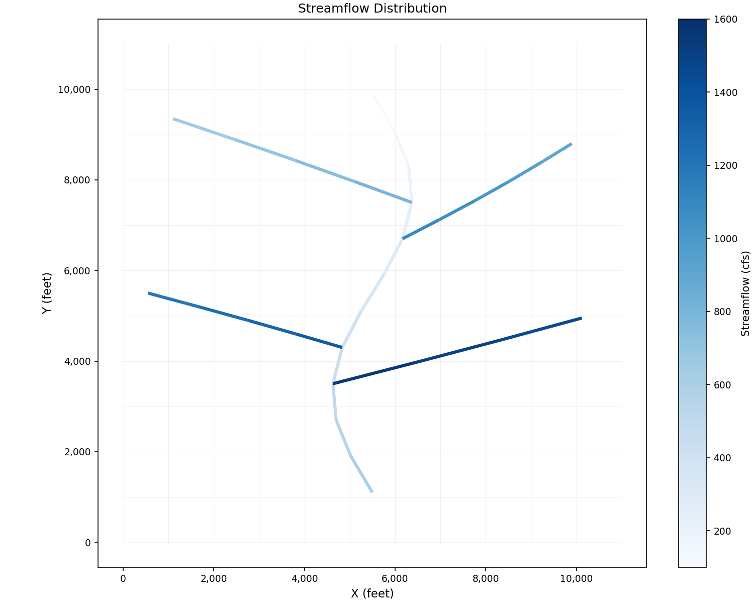
Stream Reaches with Flow Values#
Color stream reaches by flow values. When working with a full model, use
plot_streams_colored():
from pyiwfm.visualization.plotting import plot_streams_colored
import numpy as np

flow_values = np.array([...])  # one value per reach
fig, ax = plot_streams_colored(grid, model.streams, flow_values,
                                cmap='Blues', colorbar_label='Streamflow (cfs)')
plt.show()
With synthetic data using raw matplotlib:
import matplotlib.pyplot as plt
import numpy as np
from matplotlib.collections import LineCollection
from matplotlib.cm import ScalarMappable
from matplotlib.colors import Normalize
from pyiwfm.sample_models import create_sample_mesh, create_sample_stream_network
from pyiwfm.visualization.plotting import plot_mesh

mesh = create_sample_mesh(nx=12, ny=12, n_subregions=4)
stream_nodes, reaches = create_sample_stream_network(mesh)

flow_values = [100 + i * 50 for i in range(len(reaches))]

fig, ax = plot_mesh(mesh, show_edges=True, edge_color='lightgray',
                    fill_color='white', alpha=0.2)

segments = []
for from_idx, to_idx in reaches:
    x1, y1 = stream_nodes[from_idx]
    x2, y2 = stream_nodes[to_idx]
    segments.append([(x1, y1), (x2, y2)])

norm = Normalize(vmin=min(flow_values), vmax=max(flow_values))
lc = LineCollection(segments, cmap='Blues', norm=norm, linewidths=3, zorder=3)
lc.set_array(np.array(flow_values))
ax.add_collection(lc)

sm = ScalarMappable(cmap='Blues', norm=norm)
sm.set_array([])
plt.colorbar(sm, ax=ax, label='Streamflow (cfs)')

ax.autoscale()
ax.set_title('Streamflow Distribution')
ax.set_xlabel('X (feet)')
ax.set_ylabel('Y (feet)')
plt.show()
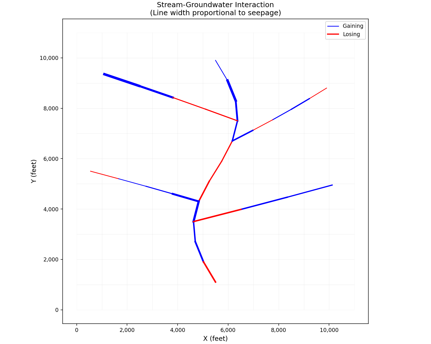
Stream-Groundwater Interaction#
Show gaining and losing reaches. With a full model, use
plot_streams_colored() with a
diverging colormap:
from pyiwfm.visualization.plotting import plot_streams_colored

fig, ax = plot_streams_colored(grid, model.streams, seepage_values,
                                cmap='RdBu', colorbar_label='Seepage (AF/day)')
plt.show()
With synthetic data:
import matplotlib.pyplot as plt
import numpy as np
from pyiwfm.sample_models import create_sample_mesh, create_sample_stream_network
from pyiwfm.visualization.plotting import plot_mesh

mesh = create_sample_mesh(nx=12, ny=12, n_subregions=4)
stream_nodes, reaches = create_sample_stream_network(mesh)

np.random.seed(42)
seepage = np.random.uniform(-50, 100, len(reaches))

fig, ax = plot_mesh(mesh, show_edges=True, edge_color='lightgray',
                    fill_color='white', alpha=0.2)

gaining_plotted = False
losing_plotted = False
for i, (from_idx, to_idx) in enumerate(reaches):
    x1, y1 = stream_nodes[from_idx]
    x2, y2 = stream_nodes[to_idx]

    if seepage[i] > 0:
        color = 'blue'
        label = 'Gaining' if not gaining_plotted else None
        gaining_plotted = True
    else:
        color = 'red'
        label = 'Losing' if not losing_plotted else None
        losing_plotted = True

    width = 1 + abs(seepage[i]) / 30
    ax.plot([x1, x2], [y1, y2], color=color, linewidth=width,
            zorder=3, label=label)

ax.legend(loc='upper right')
ax.set_title('Stream-Groundwater Interaction\n(Line width proportional to seepage)')
ax.set_xlabel('X (feet)')
ax.set_ylabel('Y (feet)')
plt.show()
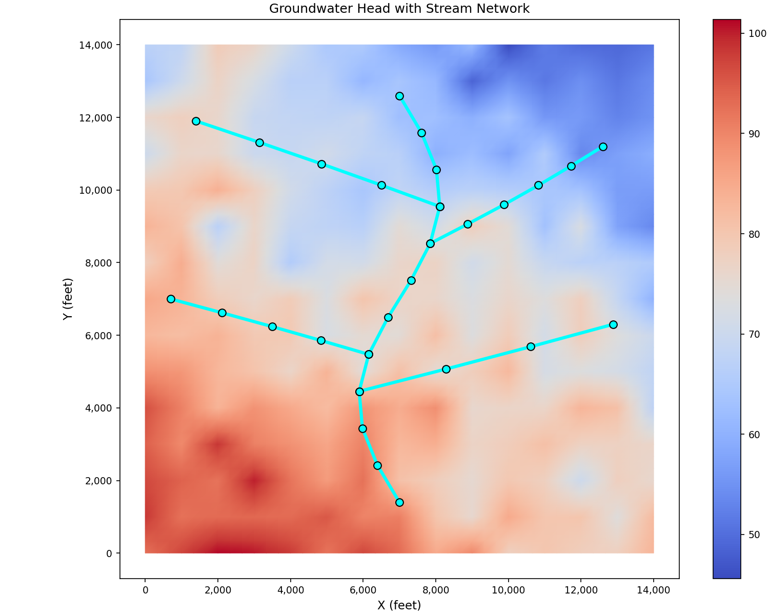
Combined Stream and Scalar Visualization#
Overlay stream network on groundwater head:
import matplotlib.pyplot as plt
from pyiwfm.sample_models import (
    create_sample_mesh, create_sample_stream_network,
    create_sample_scalar_field
)
from pyiwfm.visualization.plotting import plot_scalar_field

mesh = create_sample_mesh(nx=15, ny=15, n_subregions=4)
stream_nodes, reaches = create_sample_stream_network(mesh)
head = create_sample_scalar_field(mesh, field_type='head')

fig, ax = plot_scalar_field(mesh, head, cmap='coolwarm', show_mesh=False)

for from_idx, to_idx in reaches:
    x1, y1 = stream_nodes[from_idx]
    x2, y2 = stream_nodes[to_idx]
    ax.plot([x1, x2], [y1, y2], 'cyan', linewidth=3, zorder=3)

sx, sy = zip(*stream_nodes)
ax.scatter(sx, sy, c='cyan', s=50, edgecolor='black', zorder=4)

ax.set_title('Groundwater Head with Stream Network')
ax.set_xlabel('X (feet)')
ax.set_ylabel('Y (feet)')
plt.show()